Exploring neural cell types in ASD#
We will perform group and individual-level gene (“X”)-set enrichment analyses on autism spectrum disorder (ASD) case-control data.
First, we will fetch a parcellated ABIDE-I resting-state brain activity dataset, shipped as an example dataset with NiSpace. Additionally, we will download some t-maps published by a prior study looking at replicability of case-control differences in ASD. As reference dataset, we will use the Allen Brain Atlas gene expression data with a cell type marker collection included with NiSpace.
After covariate regression and site-harmonization, we will perform X-set enrichment colocalization analyses on an ABIDE cohort-level alteration map as well as on alteration maps for each individual ASD subject. Analyses on the downloaded t-maps serve to demonstrate replicability of our results.
[1]:
# general imports
import numpy as np
import pandas as pd
import matplotlib.pyplot as plt

# monkey patch to make progress bars show as ASCII instead of as widgets
import tqdm.notebook
tqdm.notebook.tqdm = tqdm.tqdm
[2]:
# load local nispace, for testing
# COMMENT THIS OUT IF YOU RUN THIS LOCALLY AFTER INSTALLING NISPACE
import sys
sys.path.append("/Users/llotter/projects/nispace/")
Fetch the ABIDE I example dataset#
The ABIDE I dataset shipped with NiSpace contains parcellated degree centrality data (Schaefer200 and TianS1) downloaded using nilearn’s fetch_abide_pcp() function. See the API documentation for detailed info.
[3]:
from nispace.datasets import fetch_example

# parcellation to use
parc_name = "Schaefer200"

# fetch the parcellated data and corresponding phenotypic info
abide_data, abide_pheno = fetch_example("abide", parc_name)
display(abide_pheno.shape, abide_pheno.head(5))
display(abide_data.shape, abide_data.head(5))


# get ABIDE groups: column 'dx' in the pheno data; for clarity, we use a numeric vector with
# ASD = 0 and CTRL = 1.
abide_groups = abide_pheno.dx.map({"ASD": 0, "CTRL": 1}).to_list()
INFO | 15/06/25 16:13:20 | nispace: Loading example dataset: 'abide', parcellated with: Schaefer200.
INFO | 15/06/25 16:13:20 | nispace: Returning parcellated and associated subject data.
(871, 18)
| site | site_num | dx | dx_num | dsm_iv_tr | age | sex | sex_num | qc_rater_1 | qc_func_rater_2 | qc_func_rater_3 | adi_r_social_total_a | adi_r_verbal_total_bv | adi_rrb_total_c | ados_total | srs_raw_total | scq_total | aq_total | |
|---|---|---|---|---|---|---|---|---|---|---|---|---|---|---|---|---|---|---|
| subject | ||||||||||||||||||
| 50003 | PITT | 9 | ASD | 1 | 1.0 | 24.45 | M | 1 | OK | OK | OK | 27.0 | 22.0 | 5.0 | 13.0 | NaN | NaN | NaN |
| 50004 | PITT | 9 | ASD | 1 | 1.0 | 19.09 | M | 1 | OK | OK | OK | 19.0 | 12.0 | 5.0 | 18.0 | NaN | NaN | NaN |
| 50005 | PITT | 9 | ASD | 1 | 1.0 | 13.73 | F | 2 | OK | maybe | OK | 23.0 | 19.0 | 3.0 | 12.0 | NaN | NaN | NaN |
| 50006 | PITT | 9 | ASD | 1 | 1.0 | 13.37 | M | 1 | OK | maybe | OK | 13.0 | 10.0 | 4.0 | 12.0 | NaN | NaN | NaN |
| 50007 | PITT | 9 | ASD | 1 | 1.0 | 17.78 | M | 1 | OK | maybe | OK | 21.0 | 14.0 | 9.0 | 17.0 | NaN | NaN | NaN |
(871, 200)
| hemi-L_div-Vis_lab-1 | hemi-L_div-Vis_lab-2 | hemi-L_div-Vis_lab-3 | hemi-L_div-Vis_lab-4 | hemi-L_div-Vis_lab-5 | hemi-L_div-Vis_lab-6 | hemi-L_div-Vis_lab-7 | hemi-L_div-Vis_lab-8 | hemi-L_div-Vis_lab-9 | hemi-L_div-Vis_lab-10 | ... | hemi-R_div-Default_lab-PFCm+1 | hemi-R_div-Default_lab-PFCm+2 | hemi-R_div-Default_lab-PFCm+3 | hemi-R_div-Default_lab-PFCm+4 | hemi-R_div-Default_lab-PFCm+5 | hemi-R_div-Default_lab-PFCm+6 | hemi-R_div-Default_lab-PFCm+7 | hemi-R_div-Default_lab-PCC+1 | hemi-R_div-Default_lab-PCC+2 | hemi-R_div-Default_lab-PCC+3 | |
|---|---|---|---|---|---|---|---|---|---|---|---|---|---|---|---|---|---|---|---|---|---|
| subject | |||||||||||||||||||||
| 50003 | 1530.1179 | 1677.4820 | 1607.0056 | 1508.5145 | 1187.09780 | 1510.6517 | 1534.3547 | 1513.21020 | 1557.09070 | 1394.90080 | ... | 1035.8574 | 1288.5192 | 1401.46080 | 1274.3520 | 1046.5576 | 1203.9425 | 1172.5999 | 1359.5068 | 1299.9420 | 1430.0234 |
| 50004 | 1077.5151 | 1094.0139 | 1033.4298 | 1036.3722 | 686.27716 | 1194.0590 | 917.2903 | 1004.15094 | 813.08685 | 1002.22266 | ... | 973.7754 | 1164.9417 | 905.02610 | 1122.3805 | 1072.1533 | 1013.6818 | 1072.7695 | 1255.3365 | 1186.0830 | 1342.4990 |
| 50005 | 1287.0707 | 1186.0944 | 1024.3271 | 1388.4406 | 814.70250 | 1461.1589 | 1083.4020 | 1166.30380 | 946.10547 | 1254.68530 | ... | 1491.0910 | 1365.1063 | 1056.02480 | 1367.7561 | 1115.7511 | 1207.1631 | 1180.3931 | 1568.5526 | 1548.0833 | 1324.9236 |
| 50006 | 1301.8971 | 1094.0586 | 991.6907 | 1503.6521 | 751.03217 | 1558.8677 | 1003.2750 | 1206.68430 | 955.63060 | 1779.52200 | ... | 1392.2349 | 1394.3527 | 1011.90173 | 1335.2821 | 1136.7335 | 1288.5624 | 1235.9653 | 1587.9417 | 1706.6691 | 1555.8801 |
| 50007 | 1503.5083 | 1181.2339 | 1113.0653 | 1403.4066 | 838.12440 | 1385.6886 | 1114.9324 | 1288.69320 | 946.09924 | 1222.88730 | ... | 1325.6752 | 1330.0748 | 1002.28436 | 1297.8367 | 1221.0618 | 1422.1914 | 1304.0887 | 1434.1088 | 1766.3740 | 1810.9355 |
5 rows × 200 columns
Fetch multi-cohort ASD t-maps from Holiga et al., 2019#
We download cohort-level t-maps, contrasting ASD vs. control participants in four independent cohorts: “Patients with autism spectrum disorders display reproducible functional connectivity alterations”. The data is on neurovault so we can use nilearn’s fetch_neurovault_ids function.
[4]:
from nilearn.datasets import fetch_neurovault_ids

holiga_dict = fetch_neurovault_ids([5769])
holiga_data = holiga_dict["images"]

print("Downloaded files:")
display(holiga_data)

print("Names:")
holiga_labels = [dic["name"].split(" ")[-1] for dic in holiga_dict["images_meta"]]
holiga_labels
Reading local neurovault data.
Already fetched 1 image
Already fetched 2 images
Already fetched 3 images
Already fetched 4 images
4 images found on local disk.
Downloaded files:
['/Users/llotter/nilearn_data/neurovault/collection_5769/image_134189.nii.gz',
 '/Users/llotter/nilearn_data/neurovault/collection_5769/image_134190.nii.gz',
 '/Users/llotter/nilearn_data/neurovault/collection_5769/image_134191.nii.gz',
 '/Users/llotter/nilearn_data/neurovault/collection_5769/image_134188.nii.gz']
Names:
[4]:
['ABIDE2', 'EUAIMS', 'INFOR', 'ABIDE']
Fetch reference data#
We want to perform gene (“X”)-set enrichment analyses to see if resting-state fMRI alterations in ASD share spatial patterns with genetic markers of specific neural cell types. For this, we need to fetch a mRNA dataset with a cell type “collection”. There are two Allen Brain Atlas mRNA datasets: "mrna", extracted with abagen, and "magicc", published by Wagstyl et al., 2024. We will use the "magicc"
dataset. As commonly done in gene-set enrichment analyses, we will estimate non-parametric p values by evaluating colocalization (“enrichment”) patterns with randomly selected gene sets. For this, we recommend to use the "pls" colocalization method. For this, we will need to provide a “background” gene set. Here, we just use the full mRNA dataset provided with NiSpace.
[5]:
from nispace.datasets import fetch_reference

# get cell type data
ref_data = fetch_reference(
    "magicc",
    collection="CellTypesSilettiSuperclusters",
    parcellation=parc_name,
    set_size_range=(5, None),
    print_references=False
)
display(ref_data.shape, ref_data.head(5))

# get number of maps/gene markers per set/cell type
ref_data_maps_pet_set = ref_data.index.get_level_values("set").value_counts()
print(f"Between {ref_data_maps_pet_set.min()} and {ref_data_maps_pet_set.max()} maps per set")

# get all genes as background
ref_background = fetch_reference(
    "magicc", parcellation=parc_name,
    print_references=False
)
INFO | 15/06/25 16:13:20 | nispace: Loading magicc maps.
INFO | 15/06/25 16:13:20 | nispace: Applying collection filter from: /Users/llotter/nispace-data/reference/magicc/collection-CellTypesSilettiSuperclusters.collect.
INFO | 15/06/25 16:13:21 | nispace: Filtering to collection sets with between 5 and inf maps.
INFO | 15/06/25 16:13:22 | nispace: Loading data parcellated with 'Schaefer200'
(775, 200)
| hemi-L_div-Vis_lab-1 | hemi-L_div-Vis_lab-2 | hemi-L_div-Vis_lab-3 | hemi-L_div-Vis_lab-4 | hemi-L_div-Vis_lab-5 | hemi-L_div-Vis_lab-6 | hemi-L_div-Vis_lab-7 | hemi-L_div-Vis_lab-8 | hemi-L_div-Vis_lab-9 | hemi-L_div-Vis_lab-10 | ... | hemi-R_div-Default_lab-PFCm+1 | hemi-R_div-Default_lab-PFCm+2 | hemi-R_div-Default_lab-PFCm+3 | hemi-R_div-Default_lab-PFCm+4 | hemi-R_div-Default_lab-PFCm+5 | hemi-R_div-Default_lab-PFCm+6 | hemi-R_div-Default_lab-PFCm+7 | hemi-R_div-Default_lab-PCC+1 | hemi-R_div-Default_lab-PCC+2 | hemi-R_div-Default_lab-PCC+3 | ||
|---|---|---|---|---|---|---|---|---|---|---|---|---|---|---|---|---|---|---|---|---|---|---|
| set | map | |||||||||||||||||||||
| Upper-layer IT | GLP2R | 0.938 | -0.3643 | 0.11710 | -0.84100 | -1.2980 | 0.7410 | -2.1330 | -0.190300 | -1.3350 | -1.3500 | ... | 0.80900 | 1.1160 | 1.4530 | 0.3306 | 0.270 | 0.2498 | 0.5977 | 0.27100 | 0.5234 | 0.0660 |
| CBLN2 | -1.299 | -0.9900 | -0.66850 | -1.35500 | -0.9970 | -1.3890 | -1.4240 | -0.444300 | -0.8955 | -1.4260 | ... | 0.37430 | 0.6533 | 0.6045 | 1.0800 | 1.522 | 1.8130 | 1.7970 | -0.54740 | 0.1006 | 0.2527 | |
| SLCO2A1 | -1.253 | -0.8220 | 0.02815 | -1.26200 | -0.8535 | -1.4500 | -1.2295 | -0.054960 | -1.0300 | -1.1640 | ... | 0.07240 | -0.2930 | -0.6436 | 0.4770 | 0.987 | 1.1900 | 1.0490 | -0.50900 | 0.3360 | 0.7750 | |
| MUC19 | 0.712 | -0.0338 | 0.24270 | -0.08624 | -0.4900 | 0.4907 | -0.4229 | 0.014145 | -0.5527 | 0.2690 | ... | 0.02402 | -0.2253 | -0.3872 | -0.5635 | -0.699 | -0.8870 | -0.7180 | 0.41630 | 0.1522 | 0.1590 | |
| PDGFD | 0.587 | 0.5580 | 0.70600 | 0.02979 | 0.3208 | -0.1287 | -0.1342 | 0.631000 | 0.3203 | -0.2467 | ... | -0.24290 | -0.6616 | -1.2280 | -0.8438 | -1.357 | -1.4820 | -1.6110 | 0.11127 | 0.2318 | 0.4778 |
5 rows × 200 columns
Between 5 and 161 maps per set
INFO | 15/06/25 16:13:22 | nispace: Loading magicc maps.
INFO | 15/06/25 16:13:22 | nispace: Loading data parcellated with 'Schaefer200'
Initialize NiSpace#
We fit NiSpace with the prepared data.
[6]:
from nispace import NiSpace

nsp = NiSpace(
    x=ref_data,
    y=abide_data,
    z="gm",
    parcellation=parc_name,
    standardize="xyz",
    n_proc=-1,
).fit()

# we will store our results in dictionaries:
colocs, p_values, q_values = {}, {}, {}
INFO | 15/06/25 16:13:22 | nispace: *** NiSpace.fit() - Data extraction and preparation. ***
INFO | 15/06/25 16:13:22 | nispace: Loading cortex parcellation 'Schaefer200' in 'MNI152NLin2009cAsym' space.
INFO | 15/06/25 16:13:22 | nispace: Loaded integrated parcellation with pre-calculated distance matrix.
INFO | 15/06/25 16:13:22 | nispace: Checking input data for 'x' (should be, e.g., PET data):
INFO | 15/06/25 16:13:22 | nispace: Input type: DataFrame, assuming parcellated data with shape (n_files/subjects/etc, n_parcels).
INFO | 15/06/25 16:13:22 | nispace: Got 'x' data for 775 x 200 parcels.
INFO | 15/06/25 16:13:22 | nispace: Checking input data for 'y' (should be, e.g., subject data):
INFO | 15/06/25 16:13:22 | nispace: Input type: DataFrame, assuming parcellated data with shape (n_files/subjects/etc, n_parcels).
WARNING | 15/06/25 16:13:22 | nispace: Parcellated data contains nan values!
INFO | 15/06/25 16:13:22 | nispace: Got 'y' data for 871 x 200 parcels.
INFO | 15/06/25 16:13:22 | nispace: Checking input data for z (should be, e.g., grey matter data):
INFO | 15/06/25 16:13:22 | nispace: Using standard grey matter probability map as 'z' for GMV-control.
INFO | 15/06/25 16:13:22 | nispace: Loading MNI152NLin2009cAsym 'gmprob' template in '1mm' resolution.
INFO | 15/06/25 16:13:22 | nispace: Input type: list, assuming imaging data.
INFO | 15/06/25 16:13:23 | nispace: Parcellating imaging data.
Parcellating (-1 proc): 100%|██████████| 1/1 [00:00<00:00, 103.22it/s]
INFO | 15/06/25 16:13:27 | nispace: Combined across images, 0 parcel(s) had only background intensity and were set to nan ([]).
INFO | 15/06/25 16:13:27 | nispace: Got 'z' data for 1 x 200 parcels.
INFO | 15/06/25 16:13:27 | nispace: Z-standardizing 'X' data.
INFO | 15/06/25 16:13:27 | nispace: Z-standardizing 'Y' data.
INFO | 15/06/25 16:13:27 | nispace: Z-standardizing 'Z' data.
Clean the data#
[7]:
covariates = pd.DataFrame({
    "age": abide_pheno.age,
    "sex": abide_pheno.sex_num,
    "site": abide_pheno.site_num,
    "dx": abide_pheno.dx_num
})

nsp.clean_y(
    how=["between", "within"],
    covariates_between=covariates,
    covariates_within="z",
    combat=True,
    combat_keep="dx"
)
INFO | 15/06/25 16:13:27 | nispace: *** NiSpace.clean_y() - Y covariate regression. ***
INFO | 15/06/25 16:13:27 | nispace: Performing covariate regression within map/subjects (e.g., grey matter maps).
INFO | 15/06/25 16:13:27 | nispace: Using Z data for 'within' covariate regression.
Regressing within covariate(s) on Y (-1 proc): 100%|██████████| 871/871 [00:02<00:00, 322.81it/s]
INFO | 15/06/25 16:13:33 | nispace: Performing covariate regression between maps/subjects (e.g., age, sex, site).
INFO | 15/06/25 16:13:33 | nispace: Assuming 4 'between' covariate(s) for 871 maps/subjects.
Regressing 2 between covariate(s) on Y (-1 proc): 100%|██████████| 200/200 [00:00<00:00, 299.84it/s]
INFO | 15/06/25 16:13:33 | nispace: Performing combat harmonization, retaining 1 covariates.
WARNING | 15/06/25 16:13:33 | nispace: Detected missing values in Y data, which is not supported with ComBat harmonization. Missing values will be imputed with map-wise medians and replaced by nan after harmonization. CAVE: experimental feature!
[7]:
| hemi-L_div-Vis_lab-1 | hemi-L_div-Vis_lab-2 | hemi-L_div-Vis_lab-3 | hemi-L_div-Vis_lab-4 | hemi-L_div-Vis_lab-5 | hemi-L_div-Vis_lab-6 | hemi-L_div-Vis_lab-7 | hemi-L_div-Vis_lab-8 | hemi-L_div-Vis_lab-9 | hemi-L_div-Vis_lab-10 | ... | hemi-R_div-Default_lab-PFCm+1 | hemi-R_div-Default_lab-PFCm+2 | hemi-R_div-Default_lab-PFCm+3 | hemi-R_div-Default_lab-PFCm+4 | hemi-R_div-Default_lab-PFCm+5 | hemi-R_div-Default_lab-PFCm+6 | hemi-R_div-Default_lab-PFCm+7 | hemi-R_div-Default_lab-PCC+1 | hemi-R_div-Default_lab-PCC+2 | hemi-R_div-Default_lab-PCC+3 | |
|---|---|---|---|---|---|---|---|---|---|---|---|---|---|---|---|---|---|---|---|---|---|
| subject | |||||||||||||||||||||
| 50003 | 0.767105 | 1.991793 | 2.053243 | 0.103484 | 1.640125 | 0.203869 | 1.340247 | 1.127566 | 2.307621 | -0.377047 | ... | -1.019031 | -0.307629 | 1.168255 | -0.385011 | -0.712539 | -0.471329 | -0.389361 | -0.736434 | -1.286011 | -0.534864 |
| 50004 | -0.146805 | 0.728438 | 0.426873 | -1.003276 | -0.793392 | 0.582470 | -0.845015 | -0.198357 | -0.720647 | -1.220232 | ... | -0.513802 | 0.687721 | -0.506731 | 0.609091 | 1.237871 | -0.122661 | 0.653132 | 0.818871 | 0.034415 | 1.789645 |
| 50005 | -0.535074 | -0.233028 | -0.801040 | -0.235051 | 0.037770 | 0.187071 | -0.506909 | -0.311926 | -0.207957 | -0.751612 | ... | 1.215790 | 0.028596 | -0.547970 | 0.321454 | 0.051746 | -0.304689 | -0.131534 | 0.264920 | -0.037548 | -0.680939 |
| 50006 | -0.571499 | -1.033561 | -1.166981 | -0.016373 | -0.756307 | 0.365164 | -1.419281 | -0.417169 | -0.787843 | 1.293894 | ... | 0.618754 | 0.081536 | -0.841075 | -0.095390 | -0.242263 | -0.147372 | -0.194835 | 0.448176 | 0.794168 | 0.326370 |
| 50007 | 0.300700 | -0.739301 | -0.626861 | -0.635783 | -0.458022 | -0.695749 | -1.029317 | -0.215913 | -1.039549 | -1.371744 | ... | 0.204891 | -0.286352 | -0.877480 | -0.466584 | -0.002498 | 0.321670 | -0.060829 | -0.448330 | 0.777185 | 1.204087 |
| ... | ... | ... | ... | ... | ... | ... | ... | ... | ... | ... | ... | ... | ... | ... | ... | ... | ... | ... | ... | ... | ... |
| 51583 | -0.487523 | -0.924196 | -0.404640 | -0.894917 | -0.893136 | -0.212458 | -0.965670 | 0.685146 | -1.063294 | -0.377943 | ... | 0.147877 | -0.356942 | -0.273047 | -0.335682 | -0.350246 | -0.393535 | -0.074427 | -0.375532 | -1.310685 | -0.275156 |
| 51584 | 1.463381 | 0.704586 | 1.110678 | 1.642625 | 0.907543 | 1.187444 | 2.122766 | 0.148609 | 1.668964 | 2.093428 | ... | 0.322122 | 0.581465 | 0.608568 | -0.982845 | -1.223591 | -1.825126 | -1.311661 | -0.528115 | -2.006222 | -1.658157 |
| 51585 | -0.519621 | 0.354097 | -0.652600 | 0.403236 | -0.538610 | -0.282313 | -0.333859 | -0.235908 | -0.354689 | 0.670515 | ... | -0.068095 | -0.340412 | -0.982613 | -1.065815 | -0.597045 | 0.007949 | 0.319200 | -0.665970 | -0.450181 | 0.870843 |
| 51606 | -0.474259 | -1.362292 | 0.173665 | -1.364871 | -0.398459 | -0.502568 | -1.291661 | -0.333204 | -1.032486 | -0.883120 | ... | 0.898603 | -0.191989 | -0.177004 | -0.337302 | -0.407476 | 0.738187 | 0.039377 | 1.060058 | 0.845488 | 0.460567 |
| 51607 | -0.898603 | -0.710695 | 0.337099 | -1.523676 | -0.155606 | -1.284734 | -1.301209 | -0.003485 | -0.655766 | -1.615458 | ... | 1.277432 | 0.055747 | -0.212120 | 0.527658 | 0.351737 | -0.563665 | 0.665607 | -0.727391 | 1.666485 | 1.389037 |
871 rows × 200 columns
Run colocalizations of case-control maps#
[8]:
colocalization = "pls"

for comparison in ["hedges(a,b)", "zscore(a,b)"]:
    # Transform Y
    nsp.transform_y(
        comparison,
        groups=abide_groups
    )
    # Run colocalization
    nsp.colocalize(
        colocalization,
        Y_transform=comparison,
        xsea=True
    )
    # Run permutation
    nsp.permute(
        "sets",
        colocalization,
        sets_X_background=ref_background,
        Y_transform=comparison,
        n_perm=1000
    )
    # Correct p values
    nsp.correct_p(
        mc_method="fdr",
    )
    # Save
    colocs[comparison] = nsp.get_colocalizations(method=colocalization, Y_transform=comparison)
    p_values[comparison] = nsp.get_p_values(method=colocalization, Y_transform=comparison)
    q_values[comparison] = nsp.get_p_values(method=colocalization, Y_transform=comparison, mc_method="fdrbh", norm=True)
INFO | 15/06/25 16:13:33 | nispace: *** NiSpace.transform_y() - Y transformation and comparison. ***
INFO | 15/06/25 16:13:33 | nispace: Groups/sessions vector provided, ensuring dummy-coding.
INFO | 15/06/25 16:13:33 | nispace: Applying Y transform 'hedges(a,b)'.
INFO | 15/06/25 16:13:33 | nispace: *** NiSpace.colocalize() - Estimating X & Y colocalizations. ***
INFO | 15/06/25 16:13:33 | nispace: Running 'pls' colocalization with 'hedges(a,b)' transform.
INFO | 15/06/25 16:13:33 | nispace: Will perform X-set enrichment analysis (XSEA).
INFO | 15/06/25 16:13:33 | nispace: Using 29 sets with between 5 and 161 samples. Aggregating within-set colocalizations with: mean.
INFO | 15/06/25 16:13:33 | nispace: Will regress Z from Y before colocalization calculation.
WARNING | 15/06/25 16:13:33 | nispace: It seems, Z regression was performed using NiSpace.clean_y(). Will not perform Z regression.
Colocalizing (pls, -1 proc): 100%|██████████| 1/1 [00:00<00:00, 1303.79it/s]
INFO | 15/06/25 16:13:34 | nispace: *** NiSpace.permute() - Estimate exact non-parametric p values. ***
INFO | 15/06/25 16:13:34 | nispace: Permutation of: X sets.
INFO | 15/06/25 16:13:34 | nispace: Loading transformed Y data, transform = 'hedges(a,b)'.
INFO | 15/06/25 16:13:34 | nispace: Will calculate p values for mean calculation across Y maps. Set 'p_from_average_y_coloc' = False to change this behavior.
INFO | 15/06/25 16:13:34 | nispace: Loading observed colocalizations (method = 'pls').
INFO | 15/06/25 16:13:34 | nispace: Generating permuted X sets.
INFO | 15/06/25 16:13:34 | nispace: Will use 11146 provided background maps.
INFO | 15/06/25 16:13:34 | nispace: Z-standardizing X background maps.
Permuting X set indices: 100%|██████████| 1000/1000 [00:00<00:00, 8684.09it/s]
Null colocalizations (pls, -1 proc): 100%|██████████| 1000/1000 [00:02<00:00, 340.35it/s]
INFO | 15/06/25 16:13:37 | nispace: Calculating exact p-values (tails = {'r2': 'upper', 'beta': 'two'}).
INFO | 15/06/25 16:13:37 | nispace: *** NiSpace.correct_p() - Correct p values for multiple comparisons. ***
INFO | 15/06/25 16:13:37 | nispace: Returning colocalizations:
| METHOD | XSEA | X_REDUCTION | Y_TRANSFORM |
| pls    | True | False       | hedges(a,b) |
INFO | 15/06/25 16:13:37 | nispace: Returning p values:
| METHOD | PERMUTE_WHAT | XSEA | MC_METHOD | NORM  | X_REDUCTION | Y_TRANSFORM |
| pls    | sets         | True | None      | False | False       | hedges(a,b) |
INFO | 15/06/25 16:13:37 | nispace: Returning p values:
| METHOD | PERMUTE_WHAT | XSEA | MC_METHOD | NORM | X_REDUCTION | Y_TRANSFORM |
| pls    | sets         | True | fdrbh     | True | False       | hedges(a,b) |
INFO | 15/06/25 16:13:37 | nispace: *** NiSpace.transform_y() - Y transformation and comparison. ***
INFO | 15/06/25 16:13:37 | nispace: Groups/sessions vector provided, ensuring dummy-coding.
INFO | 15/06/25 16:13:37 | nispace: Applying Y transform 'zscore(a,b)'.
INFO | 15/06/25 16:13:37 | nispace: *** NiSpace.colocalize() - Estimating X & Y colocalizations. ***
INFO | 15/06/25 16:13:37 | nispace: Running 'pls' colocalization with 'zscore(a,b)' transform.
INFO | 15/06/25 16:13:37 | nispace: Will perform X-set enrichment analysis (XSEA).
INFO | 15/06/25 16:13:37 | nispace: Using 29 sets with between 5 and 161 samples. Aggregating within-set colocalizations with: mean.
INFO | 15/06/25 16:13:37 | nispace: Will regress Z from Y before colocalization calculation.
WARNING | 15/06/25 16:13:37 | nispace: It seems, Z regression was performed using NiSpace.clean_y(). Will not perform Z regression.
Colocalizing (pls, -1 proc): 100%|██████████| 403/403 [00:01<00:00, 400.33it/s]
INFO | 15/06/25 16:13:39 | nispace: *** NiSpace.permute() - Estimate exact non-parametric p values. ***
INFO | 15/06/25 16:13:39 | nispace: Permutation of: X sets.
INFO | 15/06/25 16:13:39 | nispace: Loading transformed Y data, transform = 'zscore(a,b)'.
INFO | 15/06/25 16:13:39 | nispace: Will calculate p values for mean calculation across Y maps. Set 'p_from_average_y_coloc' = False to change this behavior.
INFO | 15/06/25 16:13:39 | nispace: Loading observed colocalizations (method = 'pls').
INFO | 15/06/25 16:13:39 | nispace: Generating permuted X sets.
INFO | 15/06/25 16:13:39 | nispace: Will use 11146 provided background maps.
INFO | 15/06/25 16:13:39 | nispace: Z-standardizing X background maps.
Permuting X set indices: 100%|██████████| 1000/1000 [00:00<00:00, 8518.03it/s]
Null colocalizations (pls, -1 proc): 100%|██████████| 1000/1000 [15:29<00:00,  1.08it/s]
INFO | 15/06/25 16:29:22 | nispace: Calculating exact p-values (tails = {'r2': 'upper', 'beta': 'two'}).
INFO | 15/06/25 16:29:22 | nispace: *** NiSpace.correct_p() - Correct p values for multiple comparisons. ***
INFO | 15/06/25 16:29:22 | nispace: Returning colocalizations:
| METHOD | XSEA | X_REDUCTION | Y_TRANSFORM |
| pls    | True | False       | zscore(a,b) |
INFO | 15/06/25 16:29:22 | nispace: Returning p values:
| METHOD | PERMUTE_WHAT | XSEA | MC_METHOD | NORM  | X_REDUCTION | Y_TRANSFORM |
| pls    | sets         | True | None      | False | False       | zscore(a,b) |
INFO | 15/06/25 16:29:22 | nispace: Returning p values:
| METHOD | PERMUTE_WHAT | XSEA | MC_METHOD | NORM | X_REDUCTION | Y_TRANSFORM |
| pls    | sets         | True | fdrbh     | True | False       | zscore(a,b) |
Replicability in Holiga2019 group-average data#
[9]:
from nispace.workflows import simple_xsea

comparison = "holiga2019"

colocs[comparison], p_values[comparison], q_values[comparison], nsp_holiga2018 = simple_xsea(
    y=holiga_data,
    x=ref_data,
    x_background=ref_background,
    z="gm",
    colocalization_method="pls",
    permute_sets=True,
    n_perm=1000,
    parcellation=parc_name,
    standardize="xyz",
    init_kwargs={"y_labels": holiga_labels},
    verbose=False,
    n_proc=-1,
    plot=False
)
INFO | 15/06/25 16:29:22 | nispace: Loading cortex parcellation 'Schaefer200' in 'MNI152NLin2009cAsym' space.
INFO | 15/06/25 16:29:22 | nispace: Loaded integrated parcellation with pre-calculated distance matrix.
INFO | 15/06/25 16:29:22 | nispace: Checking input data for 'x' (should be, e.g., PET data):
INFO | 15/06/25 16:29:23 | nispace: Loading MNI152NLin2009cAsym 'gmprob' template in '1mm' resolution.
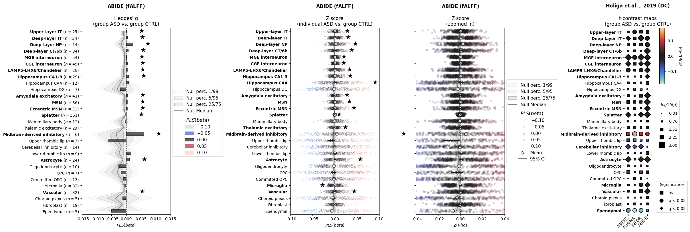
Plot results#
[10]:
from nispace.plotting import print_significance
from nispace.plotting import heatmap

fig, axes = plt.subplots(1,4, figsize=(24, 8), constrained_layout=True)


## ABIDE PLOTS

for i, (comparison, title, x_lims) in enumerate([
    ("hedges(a,b)", "$\mathbf{ABIDE\ (fALFF)}$\n\nHedges' g\n(group ASD vs. group CTRL)", (-0.015, 0.015)),
    ("zscore(a,b)", "$\mathbf{ABIDE\ (fALFF)}$\n\nZ-score\n(individual ASD vs. group CTRL)", (-0.1, 0.1)),
    ("zscore(a,b)", "$\mathbf{ABIDE\ (fALFF)}$\n\nZ-score\n(zoomed in)", (-0.04, 0.04))]):

    kwargs = {
        "fig": fig,
        "method": colocalization,
        "stats": "beta",
        "Y_transform": comparison,
        "permute_what": "sets",
        "show": False,
    }

    # plot current comparison
    nsp.plot(
        ax=axes[i],
        title=title,
        **kwargs,
        plot_kwargs={
            "legend": {
                "plot": False if i == 1 else True,
                "kwargs": {"title": "$PLS(beta)$"}
            },
            "limits": {
                "x": x_lims,
                "color": (-0.1, 0.1)
            },
            "scatters": {
                "size": 5 if i == 2 else 2
            }
        } ,
        nullplot_kwargs={
            "legend": {
                "plot": False if i == 1 else True
            }
        }
    )
    axes[i].set_xlabel("$PLS(beta)$")

    # labels for main plot
    if i in [0,1]:
        if i == 0:
            axes[i].set_yticks(
                labels=[f"{c} $(n = {ref_data_maps_pet_set[c]})$" for c in colocs[comparison]["beta"].columns],
                ticks=range(colocs[comparison]["beta"].shape[1])
            )
        print_significance(axes[i], coloc_values=colocs[comparison]["beta"], p_values=p_values[comparison]["beta"],
                           q_values=q_values[comparison]["beta"],
                           pq_positions_pad=0.005, pq_size=16)

    # no y labels for zoomed-in plot
    elif i==2:
        axes[i].set_yticklabels([])
        axes[i].set_xlabel("$Z(Rho)$")

## HOLIGA PLOT
ax = axes[-1]
ax.set_title("$\mathbf{Holiga\ et\ al.,\ 2019\ (DC)}$\n\nt-contrast maps\n(group ASD vs. group CTRL)")

significance_shapes = p_values["holiga2019"]["beta"].copy().astype(str)
significance_shapes.iloc[:] = "ns"
significance_shapes = np.where(p_values["holiga2019"]["beta"] < 0.05, "p < 0.05", significance_shapes)
significance_shapes = np.where(q_values["holiga2019"]["beta"] < 0.05, "q < 0.05", significance_shapes)

heatmap(
    ax=ax,
    data_colors=colocs["holiga2019"]["beta"].T,
    data_sizes=-np.log10(p_values["holiga2019"]["beta"].T),
    data_shapes=significance_shapes.T,
    spines=None,
    linewidth=0.02,
    ytick_labels=colocs["holiga2019"]["beta"].columns,
    xtick_labels=colocs["holiga2019"]["beta"].index,
    legend_colors_kwargs={
        "label": "$PLS(beta)$",
        "cax": ax.inset_axes((1.3, 0.7, 0.2, 0.3))
    },
    legend_sizes_kwargs={
        "title": "$-log10(p)$",
        "bbox_to_anchor": (1.1, 0.48)
    },
    legend_shapes_kwargs={
        "title": "Significance",
        "bbox_to_anchor": (1.1, 0)
    },
)

print_significance(ax,
                   p_values=p_values["holiga2019"]["beta"].min(axis=0),
                   q_values=q_values["holiga2019"]["beta"].min(axis=0))

# save
fig.savefig("abide_plot_main.pdf", bbox_inches="tight")
INFO | 15/06/25 16:29:36 | nispace: *** NiSpace.plot() - Plot colocalization results. ***
INFO | 15/06/25 16:29:36 | nispace: Creating categorical plot for method pls, colocalization stat beta.
INFO | 15/06/25 16:29:37 | nispace: *** NiSpace.plot() - Plot colocalization results. ***
INFO | 15/06/25 16:29:37 | nispace: Creating categorical plot for method pls, colocalization stat beta.
INFO | 15/06/25 16:29:37 | nispace: *** NiSpace.plot() - Plot colocalization results. ***
INFO | 15/06/25 16:29:37 | nispace: Creating categorical plot for method pls, colocalization stat beta.
[ ]: