Workflows#
NiSpace incorporates very detailed and customizable functionality to perform colocalization analyses. However, to provide an quick-and-easy access, we defined “workflow” functions that perform complete colocalization pipelines with only one command. These include:
nispace.workflows.simple_colocalization():nispace.workflows.group_comparison():nispace.workflows.simple_xsea():[13]:
# monkey patch to make progress bars show as ASCII instead of as widgets
import tqdm.notebook
tqdm.notebook.tqdm = tqdm.tqdm
[14]:
# load local nispace, for testing
# COMMENT THIS OUT IF YOU RUN THIS LOCALLY AFTER INST
import sys
sys.path.append("/Users/llotter/projects/nispace/")
Simple colocalization#
The simplest case would be: You have a group-level results map, for example a SPM t-contrast map, and are interested in whether this map (i.e., the group or session differences) is associated with neurotransmitter receptor distributions. The workflow function simple_colocalization() will take your results map and a reference dataset of neurotransmitter receptor maps as input, return the colocalization statistics including non-parametric p values, and visualize the results. Internally, this
is just calling the individual NiSpace functions in order.
Here, we use an ENIGMA cortical thickness effect size map (Cohen’s d) from a bipolar disorder case-control comparisons as our input (“target”) map. ENIGMA data are available in the 68-parcel cortical Desikan-Killiany parcellation. Of note, this would also work when passing a 2d dataframe is input (i.e., parcels in the columns, and different maps in the rows). It also works with a list of images as input.
[15]:
from nispace.datasets import fetch_example

# get the example
example_enigma_full = fetch_example("enigma", "DesikanKilliany")
print("A pd.DataFrame with disorder-vs.-control effect sizes for 68 Desikan-Killiany parcels:")
display(example_enigma_full.head(5))

# only keep the Bipolar Disorder map
example_enigma = example_enigma_full.loc["BD"]
print("A pd.Series with SCZ-vs.-control effect sizes for 68 Desikan-Killiany parcels:")
display(example_enigma)
INFO | 15/06/25 16:01:22 | nispace: Loading example dataset: 'enigma', parcellated with: DesikanKilliany.
A pd.DataFrame with disorder-vs.-control effect sizes for 68 Desikan-Killiany parcels:
| L_bankssts | L_caudalanteriorcingulate | L_caudalmiddlefrontal | L_cuneus | L_entorhinal | L_fusiform | L_inferiorparietal | L_inferiortemporal | L_isthmuscingulate | L_lateraloccipital | ... | R_rostralanteriorcingulate | R_rostralmiddlefrontal | R_superiorfrontal | R_superiorparietal | R_superiortemporal | R_supramarginal | R_frontalpole | R_temporalpole | R_transversetemporal | R_insula | |
|---|---|---|---|---|---|---|---|---|---|---|---|---|---|---|---|---|---|---|---|---|---|
| MDD | -0.058 | -0.042 | -0.014 | 0.047 | -0.041 | -0.117 | -0.063 | -0.049 | -0.104 | -0.023 | ... | -0.098 | -0.038 | -0.078 | 0.032 | -0.031 | -0.053 | -0.062 | 0.013 | -0.051 | -0.115 |
| PTSD | -0.100 | -0.100 | -0.120 | -0.070 | 0.050 | -0.060 | -0.140 | -0.070 | -0.020 | -0.150 | ... | 0.010 | -0.100 | -0.120 | -0.120 | -0.140 | -0.150 | -0.100 | -0.020 | -0.050 | -0.110 |
| AN | -0.738 | -0.065 | -0.760 | -0.663 | 0.060 | -0.538 | -0.895 | -0.537 | -0.620 | -0.747 | ... | -0.003 | -0.507 | -0.722 | -0.925 | -0.522 | -0.756 | -0.332 | -0.055 | -0.258 | -0.339 |
| ADHD | 0.000 | -0.040 | -0.050 | 0.020 | -0.080 | -0.100 | 0.010 | -0.030 | 0.030 | 0.030 | ... | -0.010 | 0.000 | 0.000 | 0.010 | 0.000 | -0.020 | 0.010 | -0.120 | 0.010 | -0.050 |
| ASD | 0.000 | 0.020 | 0.050 | 0.060 | -0.150 | NaN | 0.010 | -0.050 | 0.020 | -0.010 | ... | 0.090 | 0.220 | 0.200 | -0.040 | -0.050 | -0.080 | 0.090 | -0.150 | -0.130 | -0.100 |
5 rows × 68 columns
A pd.Series with SCZ-vs.-control effect sizes for 68 Desikan-Killiany parcels:
L_bankssts                  -0.207
L_caudalanteriorcingulate   -0.095
L_caudalmiddlefrontal       -0.266
L_cuneus                    -0.056
L_entorhinal                -0.036
                             ...
R_supramarginal             -0.184
R_frontalpole               -0.102
R_temporalpole              -0.059
R_transversetemporal        -0.109
R_insula                    -0.168
Name: BD, Length: 68, dtype: float64
We could, but do not have to, pass pre-loaded reference data to simple_colocalization(). With x = "pet", it will automatically call fetch_reference("pet") internally. A collection can be passed through x_collection, defaulting to "UniqueTracers".
[16]:
from nispace.workflows import simple_colocalization

# run the analysis, plot=True will directly plot the result
colocs, p_values, q_values, nsp_object = simple_colocalization(
    x="PET",
    y=example_enigma,
    z=None, # don't control for anything on map-level
    parcellation="DesikanKilliany",
    colocalization_method="spearman", # can be any allowed method
    n_perm=10000, # 10k permutations, this is the default
    n_proc=-1, # number of processes, defaults to 1
    seed=42, # seed for reproducibility
    plot=False, # don't plot for now
)
INFO | 15/06/25 16:01:22 | nispace: Using integrated parcellation DesikanKilliany.
INFO | 15/06/25 16:01:22 | nispace: Loading integrated pet dataset as X data.
INFO | 15/06/25 16:01:22 | nispace: Using collection UniqueTracers.
INFO | 15/06/25 16:01:22 | nispace: Loading pet maps.
INFO | 15/06/25 16:01:22 | nispace: Applying collection filter from: /Users/llotter/nispace-data/reference/pet/collection-UniqueTracers.collect.
INFO | 15/06/25 16:01:22 | nispace: Loading data parcellated with 'DesikanKilliany'
The NiSpace "PET" dataset is based on openly available nuclear imaging maps largely accessed via neuromaps
(https://neuromaps-main.readthedocs.io/). If requested in the varying original spaces and resolutions (termed "MNI152",
"fsaverageOriginal", or "fsLROriginal"), the maps are downloaded directly from the source and cached locally. If, as is highly
recommended, the maps are requested in a defined space ("MNI152NLin2009cAsym", "MNI152NLin6Asym", "fsaverage", or "fsLR"),
they are downloaded from the NiSpace-data GitHub repo (find them in `~HOME/nispace-data/reference/pet/map`).
The NiSpace-hosted MNI maps were directly registered to 2mm MNI152NLin6Asym space, and transformed to 2mm MNI152NLin2009cAsym
with a pre-estimated MNI-to-MNI transformation using SynthMorph v4 (https://martinos.org/malte/synthmorph/). The resulting maps
were masked with a liberal grey matter mask generated from the Harvard-Oxford atlas and scaled from 1e-6 to 1. The scaling was
transferred from MNI to surface maps if both were available for the same source (e.g., maps from Beliveau et al.).
The accompanying metadata table contains detailed information about tracers, source samples, original publications and data
sources, as well as the publication licenses. Every map should be cited when used. The responsibility for this lies with the user!
We additionally ask to cite:
- Markello et al., 2022 (https://doi.org/10.1038/s41592-022-01625-w)
- Hansen et al., 2022 (https://doi.org/10.1038/s41593-022-01186-3)
- Dukart et al., 2021 (https://doi.org/10.1002/hbm.25244)
- Hoffmann et al., 2024 (https://doi.org/10.1162/imag_a_00197; if NiSpace-processed maps are used)
To ensure reproducibility, note the NiSpace commit/version: 2cb3a7f5c1cea6417fe7613465a1c503f77c87c6

- target-5HT1a_tracer-way100635_n-35_dx-hc_pub-savli2012         Source: Savli2012          CC BY-NC-SA 4.0  https://doi.org/10.1016/j.neuroimage.2012.07.001
- target-5HT1b_tracer-p943_n-23_dx-hc_pub-savli2012              Source: Savli2012          CC BY-NC-SA 4.0  https://doi.org/10.1016/j.neuroimage.2012.07.001
- target-5HT2a_tracer-altanserin_n-19_dx-hc_pub-savli2012        Source: Savli2012          CC BY-NC-SA 4.0  https://doi.org/10.1016/j.neuroimage.2012.07.001
- target-5HT4_tracer-sb207145_n-59_dx-hc_pub-beliveau2017        Source: Beliveau2017       CC BY-NC-SA 4.0  https://doi.org/10.1523/JNEUROSCI.2830-16.2016
    CAVE: Processed in fsaverage space, use  volumetric maps only for subcortex! (NiSpace tables contain only fsaverage-cortical data for now.)
- target-5HT6_tracer-gsk215083_n-30_dx-hc_pub-radhakrishnan2018  Source: Radhakrishnan2018  CC BY-NC-SA 4.0  https://doi.org/10.2967/jnumed.117.206516, https://doi.org/10.1016/j.pscychresns.2019.111007
- target-5HTT_tracer-dasb_n-18_dx-hc_pub-savli2012               Source: Savli2012          CC BY-NC-SA 4.0  https://doi.org/10.1016/j.neuroimage.2012.07.001
- target-A4B2_tracer-flubatine_n-30_dx-hc_pub-hillmer2016        Source: Hillmer2016        CC BY-NC-SA 4.0  https://doi.org/10.1016/j.neuroimage.2016.07.026, https://doi.org/10.1093/ntr/ntx091
- target-CB1_tracer-omar_n-77_dx-hc_pub-normandin2015            Source: Normandin2015      CC BY-NC-SA 4.0  https://doi.org/10.1038/jcbfm.2015.46, https://doi.org/10.1016/j.bpsc.2015.09.008, https://doi.org/10.1016/j.biopsych.2015.08.021, https://doi.org/10.1111/j.1530-0277.2012.01815.x
- target-CMRglu_tracer-fdg_n-20_dx-hc_pub-castrillon2023         Source: Castrillon2023     CC BY-NC-SA 4.0  https://doi.org/10.1126/sciadv.adi7632
- target-COX1_tracer-ps13_n-11_dx-hc_pub-kim2020                 Source: Kim2020            CC0 1.0          https://doi.org/10.1007/s00259-020-04855-2, https://doi.org/10.18112/openneuro.ds004401.v1.0.1
- target-D1_tracer-sch23390_n-13_dx-hc_pub-kaller2017            Source: Kaller2017         CC BY-NC-SA 4.0  https://doi.org/10.1007/s00259-017-3645-0
- target-D23_tracer-flb457_n-55_dx-hc_pub-sandiego2015           Source: Sandiego2015       CC BY-NC-SA 4.0  https://doi.org/10.1038/jcbfm.2014.237, https://doi.org/10.1177/0271678X17737693, https://doi.org/10.1038/s41386-019-0456-y, https://doi.org/10.1001/jamapsychiatry.2014.2414, https://doi.org/10.1038/npp.2017.223
- target-DAT_tracer-fpcit_n-174_dx-hc_pub-dukart2018             Source: Dukart2018         CC BY-NC-SA 4.0  https://doi.org/10.1038/s41598-018-22444-0
    CAVE: SPECT, not PET!
- target-FDOPA_tracer-fluorodopa_n-12_dx-hc_pub-garciagomez2018  Source: Garciagomez2018    free             https://doi.org/10.33588/imagendiagnostica.901.2
- target-GABAa_tracer-flumazenil_n-6_dx-hc_pub-dukart2018        Source: Dukart2018         CC BY-NC-SA 4.0  https://doi.org/10.1038/s41598-018-22444-0
- target-GABAa5_tracer-ro154513_n-10_dx-hc_pub-lukow2022         Source: Lukow2022          CC BY 4.0        https://doi.org/10.1038/s42003-022-03268-1
- target-H3_tracer-gsk189254_n-8_dx-hc_pub-gallezot2017          Source: Gallezot2017       CC BY-NC-SA 4.0  https://doi.org/10.1177/0271678X16650697, https://doi.org/10.1038/jcbfm.2009.195
- target-HDAC_tracer-martinostat_n-8_dx-hc_pub-wey2016           Source: Wey2016            CC0 1.0          https://doi.org/10.1126/scitranslmed.aaf7551
- target-KOR_tracer-ly2795050_n-28_dx-hc_pub-vijay2018           Source: Vijay2018          CC BY-NC-SA 4.0  https://doi.org/10.1038/s41386-018-0199-1
- target-M1_tracer-lsn3172176_n-24_dx-hc_pub-naganawa2020        Source: Naganawa2020       CC BY-NC-SA 4.0  https://doi.org/10.2967/jnumed.120.246967
- target-mGluR5_tracer-abp688_n-73_dx-hc_pub-smart2019           Source: Smart2019          CC BY-NC-SA 4.0  https://doi.org/10.1007/s00259-018-4252-4
- target-MOR_tracer-carfentanil_n-204_dx-hc_pub-kantonen2020     Source: Kantonen2020       CC BY-NC-SA 4.0  https://doi.org/10.1038/mp.2017.183
- target-NET_tracer-mrb_n-10_dx-hc_pub-hesse2017                 Source: Hesse2017          CC BY-NC-SA 4.0  https://doi.org/10.1007/s00259-016-3590-3
- target-NMDA_tracer-ge179_n-29_dx-hc_pub-galovic2021            Source: Galovic2021        CC BY-NC-SA 4.0  https://doi.org/10.1001/jamaneurol.2022.4352, https://doi.org/10.1016/j.neuroimage.2021.118194, https://doi.org/10.2967/jnumed.113.130641
    CAVE: Unlike other tracers, [18F]GE-179 binds to open (active) NMDA receptors!
- target-SV2A_tracer-ucbj_n-76_dx-hc_pub-finnema2016             Source: Finnema2016        CC BY-NC-SA 4.0  https://doi.org/10.1177/0271678X17724947, https://doi.org/10.2967/jnumed.120.246967, https://doi.org/10.1177/0271678X211004312, https://doi.org/10.1186/s13195-020-00742-y, https://doi.org/10.1177/0271678X20946198, https://doi.org/10.1093/cid/ciab484, https://doi.org/10.1038/s41380-021-01184-0, https://doi.org/10.1016/j.bpsc.2015.09.008, https://doi.org/10.1111/epi.16653, https://doi.org/10.1186/s13550-020-00670-w, https://doi.org/10.1002/alz.12097, https://doi.org/10.1111/epi.14701, https://doi.org/10.1038/s41467-019-09562-7, https://doi.org/10.1001/jamaneurol.2018.1836
- target-TSPO_tracer-pbr28_n-6_dx-hc_pub-lois2018                Source: Lois2018           MIT              https://doi.org/10.1021/acschemneuro.8b00072, https://doi.org/10.5281/zenodo.1174364
- target-VAChT_tracer-feobv_n-18_dx-hc_pub-aghourian2017         Source: Aghourian2017      CC BY-NC-SA 4.0  https://doi.org/10.1038/mp.2017.183
- target-VMAT2_tracer-dtbz_n-76_dx-hc_pub-larsen2020             Source: Larsen2020         CC0 1.0          https://doi.org/10.18112/openneuro.ds002385.v1.1.0, https://doi.org/10.1038/s41467-020-14693-3

INFO | 15/06/25 16:01:22 | nispace: *** NiSpace.fit() - Data extraction and preparation. ***
INFO | 15/06/25 16:01:22 | nispace: Loading cortex parcellation 'DesikanKilliany' in 'MNI152NLin2009cAsym' space.
INFO | 15/06/25 16:01:22 | nispace: Loaded integrated parcellation with pre-calculated distance matrix.
INFO | 15/06/25 16:01:22 | nispace: Checking input data for 'x' (should be, e.g., PET data):
INFO | 15/06/25 16:01:22 | nispace: Input type: DataFrame, assuming parcellated data with shape (n_files/subjects/etc, n_parcels).
WARNING | 15/06/25 16:01:22 | nispace: Parcellated data contains nan values!
INFO | 15/06/25 16:01:22 | nispace: Got 'x' data for 28 x 68 parcels.
INFO | 15/06/25 16:01:22 | nispace: Checking input data for 'y' (should be, e.g., subject data):
INFO | 15/06/25 16:01:22 | nispace: Input type: Series, assuming parcellated data with shape (1, n_parcels).
INFO | 15/06/25 16:01:22 | nispace: Got 'y' data for 1 x 68 parcels.
INFO | 15/06/25 16:01:22 | nispace: Z-standardizing 'X' data.
INFO | 15/06/25 16:01:22 | nispace: *** NiSpace.colocalize() - Estimating X & Y colocalizations. ***
INFO | 15/06/25 16:01:22 | nispace: Running 'spearman' colocalization.
Colocalizing (spearman, -1 proc): 100%|██████████| 1/1 [00:00<00:00, 1310.31it/s]
INFO | 15/06/25 16:01:22 | nispace: *** NiSpace.permute() - Estimate exact non-parametric p values. ***
INFO | 15/06/25 16:01:22 | nispace: Permutation of: X maps.
INFO | 15/06/25 16:01:22 | nispace: Loading observed colocalizations (method = 'spearman').
INFO | 15/06/25 16:01:22 | nispace: Generating permuted X maps.
INFO | 15/06/25 16:01:22 | nispace: No null maps found.
INFO | 15/06/25 16:01:22 | nispace: Generating null maps (n = 10000, null_method = 'moran').
INFO | 15/06/25 16:01:22 | nispace: Null map generation: Assuming n = 28 data vector(s) for n = 68 parcels.
INFO | 15/06/25 16:01:22 | nispace: Using provided distance matrix/matrices.
INFO | 15/06/25 16:01:22 | nispace: Generating null data separately for left and right hemisphere.
Moran null maps (-1 proc): 100%|██████████| 28/28 [00:00<00:00, 290.28it/s]
INFO | 15/06/25 16:01:22 | nispace: Left-to-right mirroring null maps (simple mirroring).
INFO | 15/06/25 16:01:22 | nispace: Matching interhemispheric correlation. Observed correlation: 0.96 (mean), 0.83 - 1.00 (range)
Mirroring null maps: 100%|██████████| 28/28 [00:00<00:00, 219.40it/s]
INFO | 15/06/25 16:01:23 | nispace: Null data generation finished.
INFO | 15/06/25 16:01:23 | nispace: Z-standardizing null maps.
Null colocalizations (spearman, -1 proc): 100%|██████████| 10000/10000 [00:00<00:00, 19432.31it/s]
INFO | 15/06/25 16:01:24 | nispace: Calculating exact p-values (tails = {'rho': 'two'}).
INFO | 15/06/25 16:01:24 | nispace: *** NiSpace.correct_p() - Correct p values for multiple comparisons. ***
INFO | 15/06/25 16:01:24 | nispace: Returning colocalizations:
| METHOD   | XSEA  | X_REDUCTION | Y_TRANSFORM |
| spearman | False | False       | False       |
INFO | 15/06/25 16:01:24 | nispace: Returning p values:
| METHOD   | PERMUTE_WHAT | XSEA  | MC_METHOD | NORM  | X_REDUCTION | Y_TRANSFORM |
| spearman | xmaps        | False | None      | False | False       | False       |
INFO | 15/06/25 16:01:24 | nispace: Returning p values:
| METHOD   | PERMUTE_WHAT | XSEA  | MC_METHOD | NORM  | X_REDUCTION | Y_TRANSFORM |
| spearman | xmaps        | False | fdrbh     | False | False       | False       |
Results will be 2d dataframes with Spearman coefficients, p-values, and q-values. The dataframes will have shape (1,n_parcels) as we passed one map only. We concatenate them for nice display:
[17]:
import pandas as pd

# concatenate
simple_results = pd.concat([colocs, p_values, q_values], keys=["rho", "p", "q"])
# reorder levels
simple_results = simple_results.reorder_levels([1,0]).sort_index()
# show
display(simple_results.head(5))
| set | General | Immunity | Glutamate | GABA | ... | Serotonin | Noradrenaline/Acetylcholine | Opiods/Endocannabinoids | Histamine | |||||||||||||
|---|---|---|---|---|---|---|---|---|---|---|---|---|---|---|---|---|---|---|---|---|---|---|
| map | target-CMRglu_tracer-fdg_n-20_dx-hc_pub-castrillon2023 | target-SV2A_tracer-ucbj_n-76_dx-hc_pub-finnema2016 | target-HDAC_tracer-martinostat_n-8_dx-hc_pub-wey2016 | target-VMAT2_tracer-dtbz_n-76_dx-hc_pub-larsen2020 | target-TSPO_tracer-pbr28_n-6_dx-hc_pub-lois2018 | target-COX1_tracer-ps13_n-11_dx-hc_pub-kim2020 | target-mGluR5_tracer-abp688_n-73_dx-hc_pub-smart2019 | target-NMDA_tracer-ge179_n-29_dx-hc_pub-galovic2021 | target-GABAa5_tracer-ro154513_n-10_dx-hc_pub-lukow2022 | target-GABAa_tracer-flumazenil_n-6_dx-hc_pub-dukart2018 | ... | target-5HT6_tracer-gsk215083_n-30_dx-hc_pub-radhakrishnan2018 | target-5HTT_tracer-dasb_n-18_dx-hc_pub-savli2012 | target-NET_tracer-mrb_n-10_dx-hc_pub-hesse2017 | target-A4B2_tracer-flubatine_n-30_dx-hc_pub-hillmer2016 | target-M1_tracer-lsn3172176_n-24_dx-hc_pub-naganawa2020 | target-VAChT_tracer-feobv_n-18_dx-hc_pub-aghourian2017 | target-MOR_tracer-carfentanil_n-204_dx-hc_pub-kantonen2020 | target-KOR_tracer-ly2795050_n-28_dx-hc_pub-vijay2018 | target-CB1_tracer-omar_n-77_dx-hc_pub-normandin2015 | target-H3_tracer-gsk189254_n-8_dx-hc_pub-gallezot2017 | |
| BD | p | 0.801400 | 0.131600 | 0.856600 | 0.424000 | 0.404000 | 0.493000 | 0.598200 | 0.608800 | 0.979000 | 0.835000 | ... | 0.012600 | 0.143800 | 0.823000 | 0.008000 | 0.511000 | 0.897200 | 0.153400 | 0.206400 | 0.036200 | 0.414000 |
| q | 0.966215 | 0.536900 | 0.966215 | 0.848000 | 0.848000 | 0.894250 | 0.947022 | 0.947022 | 0.979000 | 0.966215 | ... | 0.117600 | 0.536900 | 0.966215 | 0.117600 | 0.894250 | 0.966215 | 0.536900 | 0.642133 | 0.230720 | 0.848000 | |
| rho | -0.052420 | -0.200253 | -0.058623 | 0.236556 | -0.188719 | 0.213636 | -0.123423 | -0.121137 | -0.010956 | 0.028484 | ... | -0.489899 | 0.544559 | 0.055215 | -0.371505 | -0.128698 | 0.062071 | -0.224795 | -0.260417 | -0.338678 | -0.180584 | |
3 rows × 28 columns
Okay, let’s look at the lowest p values for BD:
[18]:
simple_results.T.sort_values(by=("BD", "p"))
[18]:
| BD | ||||
|---|---|---|---|---|
| p | q | rho | ||
| set | map | |||
| Noradrenaline/Acetylcholine | target-A4B2_tracer-flubatine_n-30_dx-hc_pub-hillmer2016 | 0.0080 | 0.117600 | -0.371505 |
| Serotonin | target-5HT4_tracer-sb207145_n-59_dx-hc_pub-beliveau2017 | 0.0124 | 0.117600 | -0.449467 |
| target-5HT6_tracer-gsk215083_n-30_dx-hc_pub-radhakrishnan2018 | 0.0126 | 0.117600 | -0.489899 | |
| Opiods/Endocannabinoids | target-CB1_tracer-omar_n-77_dx-hc_pub-normandin2015 | 0.0362 | 0.230720 | -0.338678 |
| Serotonin | target-5HT2a_tracer-altanserin_n-19_dx-hc_pub-savli2012 | 0.0412 | 0.230720 | -0.335819 |
| General | target-SV2A_tracer-ucbj_n-76_dx-hc_pub-finnema2016 | 0.1316 | 0.536900 | -0.200253 |
| Serotonin | target-5HTT_tracer-dasb_n-18_dx-hc_pub-savli2012 | 0.1438 | 0.536900 | 0.544559 |
| Opiods/Endocannabinoids | target-MOR_tracer-carfentanil_n-204_dx-hc_pub-kantonen2020 | 0.1534 | 0.536900 | -0.224795 |
| target-KOR_tracer-ly2795050_n-28_dx-hc_pub-vijay2018 | 0.2064 | 0.642133 | -0.260417 | |
| Dopamine | target-DAT_tracer-fpcit_n-174_dx-hc_pub-dukart2018 | 0.2888 | 0.808640 | 0.350731 |
| target-D23_tracer-flb457_n-55_dx-hc_pub-sandiego2015 | 0.3942 | 0.848000 | -0.126447 | |
| Immunity | target-TSPO_tracer-pbr28_n-6_dx-hc_pub-lois2018 | 0.4040 | 0.848000 | -0.188719 |
| Histamine | target-H3_tracer-gsk189254_n-8_dx-hc_pub-gallezot2017 | 0.4140 | 0.848000 | -0.180584 |
| General | target-VMAT2_tracer-dtbz_n-76_dx-hc_pub-larsen2020 | 0.4240 | 0.848000 | 0.236556 |
| Immunity | target-COX1_tracer-ps13_n-11_dx-hc_pub-kim2020 | 0.4930 | 0.894250 | 0.213636 |
| Noradrenaline/Acetylcholine | target-M1_tracer-lsn3172176_n-24_dx-hc_pub-naganawa2020 | 0.5110 | 0.894250 | -0.128698 |
| Glutamate | target-mGluR5_tracer-abp688_n-73_dx-hc_pub-smart2019 | 0.5982 | 0.947022 | -0.123423 |
| target-NMDA_tracer-ge179_n-29_dx-hc_pub-galovic2021 | 0.6088 | 0.947022 | -0.121137 | |
| Serotonin | target-5HT1b_tracer-p943_n-23_dx-hc_pub-savli2012 | 0.6522 | 0.961137 | -0.271183 |
| target-5HT1a_tracer-way100635_n-35_dx-hc_pub-savli2012 | 0.6928 | 0.966215 | -0.100810 | |
| General | target-CMRglu_tracer-fdg_n-20_dx-hc_pub-castrillon2023 | 0.8014 | 0.966215 | -0.052420 |
| Noradrenaline/Acetylcholine | target-NET_tracer-mrb_n-10_dx-hc_pub-hesse2017 | 0.8230 | 0.966215 | 0.055215 |
| GABA | target-GABAa_tracer-flumazenil_n-6_dx-hc_pub-dukart2018 | 0.8350 | 0.966215 | 0.028484 |
| General | target-HDAC_tracer-martinostat_n-8_dx-hc_pub-wey2016 | 0.8566 | 0.966215 | -0.058623 |
| Dopamine | target-D1_tracer-sch23390_n-13_dx-hc_pub-kaller2017 | 0.8732 | 0.966215 | 0.078106 |
| Noradrenaline/Acetylcholine | target-VAChT_tracer-feobv_n-18_dx-hc_pub-aghourian2017 | 0.8972 | 0.966215 | 0.062071 |
| Dopamine | target-FDOPA_tracer-fluorodopa_n-12_dx-hc_pub-garciagomez2018 | 0.9382 | 0.972948 | 0.025848 |
| GABA | target-GABAa5_tracer-ro154513_n-10_dx-hc_pub-lukow2022 | 0.9790 | 0.979000 | -0.010956 |
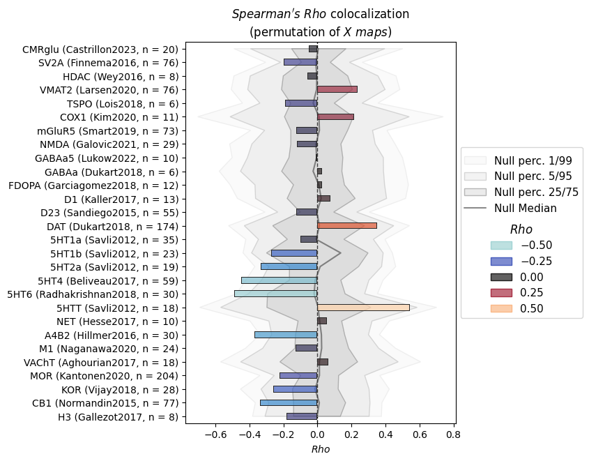
We find the strongest colocalization between cortical thickness changes in BD and and two serotonin receptors. The colocalization is negative, i.e., regions with negative effect sizes (BD < controls) have a high concentration of serotonin receptors. However, it is only marginally significant relative to null maps with a similar degree of spatial autocorrelation.
NiSpace by calling .plot("categorical") on the NiSpace instance returned by the workflow function:[19]:
fig, ax, plot = nsp_object.plot("categorical")
INFO | 15/06/25 16:01:24 | nispace: *** NiSpace.plot() - Plot colocalization results. ***
INFO | 15/06/25 16:01:25 | nispace: Creating categorical plot for method spearman, colocalization stat rho.
Group comparison#
Implemented here via nispace.workflows.group_comparison(), this is the core functionality of the MATLAB JuSpace package. The typical scenario would be: I have MRI images of two groups or sessions, which I want to compare against each other. Examples would be patients vs. controls (groups), old vs. young, (groups), the same subjects pre- vs post treatment (sessions), or during rest vs. during a task (sessions).
The approach applies the following principle: We take each subject’s image, we calculate a group/session comparison statistic for each parcel, and then we calculate colocalization statistics using the parcel-wise group/session comparison values. The last part equals the simple_colocalization() method above. However, here, we have single-subject maps, so we can permute the groups instead of the maps, which actually better fits our null hypothesis and is less conservative.
We use the ABIDE example dataset. Here, we get parcellated data (“degree centrality”) for many ASD- and control-subjects along with phenotypic information.
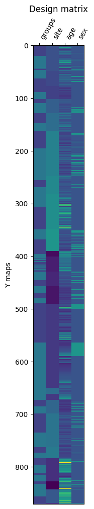
The minimum data we have to provide is the parcellated data via “x” and the group information via “design”. The framework is actually no GLM but is implemented in a GLM-style to match what people already use in neuroimaging analysis. So, the “design” should be a DataFrame with as many rows as there are subjects plus minimally a dummy column named “groups”. Another specially treated column is “site” for scanner/study site. If we pass nothing else, everything including the “site” column will be
regressed from the parcel-wise data. If we pass combat = True, ComBat harmonization will be used to remove site effects.
The group comparison method determines the output format. Following the ENIGMA example above, we can a group-level effect size ("cohen(a,b)"or "hedges(a,b)"), which will result in one group comparison map, which will be colocalized with the reference dataset. On the other hand, we can use "zscore(a,b)" to calculate z scores for every subject in group A (lowest value in the “group” design column) vs. mean and sd of group B. This will result in one map for every subject in group A,
to be colocalized with the reference dataset. While we then could calculate one p value for every subject, the default is to calculate p values for the mean of all colocalization values across group-A-subject for easier interpretation.
Let’s start with version 1 and "hedges":
[20]:
from nispace.datasets import fetch_example
from nispace.workflows import group_comparison

# parcellation, we want to use (for abide, can be Schaefer200 or Schaefer200TianS1)
parc = "Schaefer200TianS1"

# get the example
example_abide, info_abide = fetch_example("abide", parc)
print("A pd.DataFrame with single-subject values for 216 Schaefer/Melbourne parcels:")
display(example_abide)

# define the design
design = pd.DataFrame({
    "groups": info_abide["dx_num"],
    "site": info_abide["site_num"],
    "age": info_abide["age"],
    "sex": info_abide["sex_num"]
})
print("A pd.DataFrame for the design with group and site information in numerical format:")
display(design)

# run the analysis, plot=True will directly plot the result
colocs, p_values, q_values, nsp_object = group_comparison(
    x="PET",
    design=design,
    y=example_abide,
    z="gm", # control for standard gray matter probability on map-level
    parcellation=parc,
    colocalization_method="spearman", # can be any allowed method
    comparison_method="hedges(a,b)",
    n_proc=-1, # number of processes, defaults to 1
    seed=42, # seed for reproducibility
    plot=False, # don't plot for now
)
INFO | 15/06/25 16:01:26 | nispace: Loading example dataset: 'abide', parcellated with: Schaefer200TianS1.
INFO | 15/06/25 16:01:26 | nispace: Returning parcellated and associated subject data.
A pd.DataFrame with single-subject values for 216 Schaefer/Melbourne parcels:
| hemi-L_div-Vis_lab-1 | hemi-L_div-Vis_lab-2 | hemi-L_div-Vis_lab-3 | hemi-L_div-Vis_lab-4 | hemi-L_div-Vis_lab-5 | hemi-L_div-Vis_lab-6 | hemi-L_div-Vis_lab-7 | hemi-L_div-Vis_lab-8 | hemi-L_div-Vis_lab-9 | hemi-L_div-Vis_lab-10 | ... | hemi-L_lab-PUT | hemi-L_lab-CAU | hemi-R_lab-HIP | hemi-R_lab-AMY | hemi-R_lab-pTHA | hemi-R_lab-aTHA | hemi-R_lab-NAc | hemi-R_lab-GP | hemi-R_lab-PUT | hemi-R_lab-CAU | |
|---|---|---|---|---|---|---|---|---|---|---|---|---|---|---|---|---|---|---|---|---|---|
| subject | |||||||||||||||||||||
| 50003 | 1530.11790 | 1677.48200 | 1607.00560 | 1508.51450 | 1187.09780 | 1510.65170 | 1534.35470 | 1513.21020 | 1557.09070 | 1394.90080 | ... | 1288.88000 | 1246.14330 | 1061.72600 | 1057.39590 | 1185.12820 | 1366.74850 | 1374.32760 | 1028.86320 | 1220.36430 | 1366.88420 |
| 50004 | 1077.51510 | 1094.01390 | 1033.42980 | 1036.37220 | 686.27716 | 1194.05900 | 917.29030 | 1004.15094 | 813.08685 | 1002.22266 | ... | 1011.58075 | 921.38135 | 932.35223 | 891.83840 | 961.86460 | 942.36310 | 1018.32367 | 854.32776 | 956.10596 | 943.59900 |
| 50005 | 1287.07070 | 1186.09440 | 1024.32710 | 1388.44060 | 814.70250 | 1461.15890 | 1083.40200 | 1166.30380 | 946.10547 | 1254.68530 | ... | 1273.04880 | 1111.30180 | 1052.04750 | 1133.16930 | 1140.87670 | 1122.53640 | 1142.63590 | 993.38480 | 1309.49410 | 1070.89110 |
| 50006 | 1301.89710 | 1094.05860 | 991.69070 | 1503.65210 | 751.03217 | 1558.86770 | 1003.27500 | 1206.68430 | 955.63060 | 1779.52200 | ... | 1111.70310 | 1024.06250 | 1161.70690 | 1230.74290 | 1103.48690 | 1058.50400 | 929.65420 | 929.08440 | 1046.40090 | 1028.61660 |
| 50007 | 1503.50830 | 1181.23390 | 1113.06530 | 1403.40660 | 838.12440 | 1385.68860 | 1114.93240 | 1288.69320 | 946.09924 | 1222.88730 | ... | 1196.67370 | 1202.98320 | 1167.58180 | 1088.90860 | 1052.75670 | 1034.66260 | 1227.07100 | 994.04517 | 1185.00150 | 1214.71370 |
| ... | ... | ... | ... | ... | ... | ... | ... | ... | ... | ... | ... | ... | ... | ... | ... | ... | ... | ... | ... | ... | ... |
| 51583 | 535.78503 | 542.66330 | 582.85333 | 631.72095 | 392.55286 | 665.45264 | 608.18567 | 870.10120 | 513.59990 | 712.07465 | ... | 637.00260 | 599.16626 | 539.46716 | 528.19696 | 688.72107 | 696.58110 | 669.21344 | 518.96760 | 638.49840 | 582.08680 |
| 51584 | 873.60020 | 889.73230 | 879.95450 | 1139.59380 | 758.72736 | 963.26105 | 1212.34350 | 909.34094 | 1081.12320 | 1202.68650 | ... | 636.17883 | 567.40140 | 643.14840 | 738.27090 | 498.28638 | 626.71450 | 681.02014 | 603.96500 | 651.86005 | 619.42370 |
| 51585 | 841.04016 | 1076.49330 | 836.43240 | 1230.41220 | 675.63184 | 979.42910 | 1021.10890 | 1044.99200 | 909.55853 | 1283.35440 | ... | 735.39700 | 783.99603 | 650.53570 | 632.79540 | 779.42100 | 860.96260 | 686.74980 | 550.12756 | 706.34060 | 722.38120 |
| 51606 | 379.75626 | 305.59787 | 414.85750 | 352.52594 | 229.13740 | 427.65970 | 281.77176 | 414.30664 | 266.34192 | 419.60780 | ... | 304.08047 | 300.89178 | 356.77383 | 312.63156 | 336.82678 | 329.37958 | 333.69592 | 274.16850 | 301.15665 | 332.63318 |
| 51607 | 424.84604 | 463.10950 | 531.24690 | 439.38986 | 293.28760 | 430.77620 | 360.46326 | 538.20764 | 365.30743 | 430.92194 | ... | 426.81854 | 382.30450 | 373.57350 | 368.97570 | 392.87840 | 389.35010 | 246.78383 | 327.36720 | 437.44284 | 360.35666 |
871 rows × 216 columns
A pd.DataFrame for the design with group and site information in numerical format:
| groups | site | age | sex | |
|---|---|---|---|---|
| subject | ||||
| 50003 | 1 | 9 | 24.45 | 1 |
| 50004 | 1 | 9 | 19.09 | 1 |
| 50005 | 1 | 9 | 13.73 | 2 |
| 50006 | 1 | 9 | 13.37 | 1 |
| 50007 | 1 | 9 | 17.78 | 1 |
| ... | ... | ... | ... | ... |
| 51583 | 1 | 10 | 35.00 | 1 |
| 51584 | 1 | 10 | 49.00 | 1 |
| 51585 | 1 | 10 | 27.00 | 1 |
| 51606 | 1 | 5 | 29.00 | 2 |
| 51607 | 1 | 5 | 26.00 | 1 |
871 rows × 4 columns
INFO | 15/06/25 16:01:26 | nispace: Using integrated parcellation Schaefer200TianS1.
INFO | 15/06/25 16:01:26 | nispace: Loading integrated pet dataset as X data.
INFO | 15/06/25 16:01:26 | nispace: Using collection UniqueTracers.
INFO | 15/06/25 16:01:26 | nispace: Loading pet maps.
INFO | 15/06/25 16:01:26 | nispace: Applying collection filter from: /Users/llotter/nispace-data/reference/pet/collection-UniqueTracers.collect.
INFO | 15/06/25 16:01:26 | nispace: Loading and inner-merging data parcellated with 'Schaefer200' and 'TianS1'
The NiSpace "PET" dataset is based on openly available nuclear imaging maps largely accessed via neuromaps
(https://neuromaps-main.readthedocs.io/). If requested in the varying original spaces and resolutions (termed "MNI152",
"fsaverageOriginal", or "fsLROriginal"), the maps are downloaded directly from the source and cached locally. If, as is highly
recommended, the maps are requested in a defined space ("MNI152NLin2009cAsym", "MNI152NLin6Asym", "fsaverage", or "fsLR"),
they are downloaded from the NiSpace-data GitHub repo (find them in `~HOME/nispace-data/reference/pet/map`).
The NiSpace-hosted MNI maps were directly registered to 2mm MNI152NLin6Asym space, and transformed to 2mm MNI152NLin2009cAsym
with a pre-estimated MNI-to-MNI transformation using SynthMorph v4 (https://martinos.org/malte/synthmorph/). The resulting maps
were masked with a liberal grey matter mask generated from the Harvard-Oxford atlas and scaled from 1e-6 to 1. The scaling was
transferred from MNI to surface maps if both were available for the same source (e.g., maps from Beliveau et al.).
The accompanying metadata table contains detailed information about tracers, source samples, original publications and data
sources, as well as the publication licenses. Every map should be cited when used. The responsibility for this lies with the user!
We additionally ask to cite:
- Markello et al., 2022 (https://doi.org/10.1038/s41592-022-01625-w)
- Hansen et al., 2022 (https://doi.org/10.1038/s41593-022-01186-3)
- Dukart et al., 2021 (https://doi.org/10.1002/hbm.25244)
- Hoffmann et al., 2024 (https://doi.org/10.1162/imag_a_00197; if NiSpace-processed maps are used)
To ensure reproducibility, note the NiSpace commit/version: 2cb3a7f5c1cea6417fe7613465a1c503f77c87c6

- target-5HT1a_tracer-way100635_n-35_dx-hc_pub-savli2012         Source: Savli2012          CC BY-NC-SA 4.0  https://doi.org/10.1016/j.neuroimage.2012.07.001
- target-5HT1b_tracer-p943_n-23_dx-hc_pub-savli2012              Source: Savli2012          CC BY-NC-SA 4.0  https://doi.org/10.1016/j.neuroimage.2012.07.001
- target-5HT2a_tracer-altanserin_n-19_dx-hc_pub-savli2012        Source: Savli2012          CC BY-NC-SA 4.0  https://doi.org/10.1016/j.neuroimage.2012.07.001
- target-5HT4_tracer-sb207145_n-59_dx-hc_pub-beliveau2017        Source: Beliveau2017       CC BY-NC-SA 4.0  https://doi.org/10.1523/JNEUROSCI.2830-16.2016
    CAVE: Processed in fsaverage space, use  volumetric maps only for subcortex! (NiSpace tables contain only fsaverage-cortical data for now.)
- target-5HT6_tracer-gsk215083_n-30_dx-hc_pub-radhakrishnan2018  Source: Radhakrishnan2018  CC BY-NC-SA 4.0  https://doi.org/10.2967/jnumed.117.206516, https://doi.org/10.1016/j.pscychresns.2019.111007
- target-5HTT_tracer-dasb_n-18_dx-hc_pub-savli2012               Source: Savli2012          CC BY-NC-SA 4.0  https://doi.org/10.1016/j.neuroimage.2012.07.001
- target-A4B2_tracer-flubatine_n-30_dx-hc_pub-hillmer2016        Source: Hillmer2016        CC BY-NC-SA 4.0  https://doi.org/10.1016/j.neuroimage.2016.07.026, https://doi.org/10.1093/ntr/ntx091
- target-CB1_tracer-omar_n-77_dx-hc_pub-normandin2015            Source: Normandin2015      CC BY-NC-SA 4.0  https://doi.org/10.1038/jcbfm.2015.46, https://doi.org/10.1016/j.bpsc.2015.09.008, https://doi.org/10.1016/j.biopsych.2015.08.021, https://doi.org/10.1111/j.1530-0277.2012.01815.x
- target-CMRglu_tracer-fdg_n-20_dx-hc_pub-castrillon2023         Source: Castrillon2023     CC BY-NC-SA 4.0  https://doi.org/10.1126/sciadv.adi7632
- target-COX1_tracer-ps13_n-11_dx-hc_pub-kim2020                 Source: Kim2020            CC0 1.0          https://doi.org/10.1007/s00259-020-04855-2, https://doi.org/10.18112/openneuro.ds004401.v1.0.1
- target-D1_tracer-sch23390_n-13_dx-hc_pub-kaller2017            Source: Kaller2017         CC BY-NC-SA 4.0  https://doi.org/10.1007/s00259-017-3645-0
- target-D23_tracer-flb457_n-55_dx-hc_pub-sandiego2015           Source: Sandiego2015       CC BY-NC-SA 4.0  https://doi.org/10.1038/jcbfm.2014.237, https://doi.org/10.1177/0271678X17737693, https://doi.org/10.1038/s41386-019-0456-y, https://doi.org/10.1001/jamapsychiatry.2014.2414, https://doi.org/10.1038/npp.2017.223
- target-DAT_tracer-fpcit_n-174_dx-hc_pub-dukart2018             Source: Dukart2018         CC BY-NC-SA 4.0  https://doi.org/10.1038/s41598-018-22444-0
    CAVE: SPECT, not PET!
- target-FDOPA_tracer-fluorodopa_n-12_dx-hc_pub-garciagomez2018  Source: Garciagomez2018    free             https://doi.org/10.33588/imagendiagnostica.901.2
- target-GABAa_tracer-flumazenil_n-6_dx-hc_pub-dukart2018        Source: Dukart2018         CC BY-NC-SA 4.0  https://doi.org/10.1038/s41598-018-22444-0
- target-GABAa5_tracer-ro154513_n-10_dx-hc_pub-lukow2022         Source: Lukow2022          CC BY 4.0        https://doi.org/10.1038/s42003-022-03268-1
- target-H3_tracer-gsk189254_n-8_dx-hc_pub-gallezot2017          Source: Gallezot2017       CC BY-NC-SA 4.0  https://doi.org/10.1177/0271678X16650697, https://doi.org/10.1038/jcbfm.2009.195
- target-HDAC_tracer-martinostat_n-8_dx-hc_pub-wey2016           Source: Wey2016            CC0 1.0          https://doi.org/10.1126/scitranslmed.aaf7551
- target-KOR_tracer-ly2795050_n-28_dx-hc_pub-vijay2018           Source: Vijay2018          CC BY-NC-SA 4.0  https://doi.org/10.1038/s41386-018-0199-1
- target-M1_tracer-lsn3172176_n-24_dx-hc_pub-naganawa2020        Source: Naganawa2020       CC BY-NC-SA 4.0  https://doi.org/10.2967/jnumed.120.246967
- target-mGluR5_tracer-abp688_n-73_dx-hc_pub-smart2019           Source: Smart2019          CC BY-NC-SA 4.0  https://doi.org/10.1007/s00259-018-4252-4
- target-MOR_tracer-carfentanil_n-204_dx-hc_pub-kantonen2020     Source: Kantonen2020       CC BY-NC-SA 4.0  https://doi.org/10.1038/mp.2017.183
- target-NET_tracer-mrb_n-10_dx-hc_pub-hesse2017                 Source: Hesse2017          CC BY-NC-SA 4.0  https://doi.org/10.1007/s00259-016-3590-3
- target-NMDA_tracer-ge179_n-29_dx-hc_pub-galovic2021            Source: Galovic2021        CC BY-NC-SA 4.0  https://doi.org/10.1001/jamaneurol.2022.4352, https://doi.org/10.1016/j.neuroimage.2021.118194, https://doi.org/10.2967/jnumed.113.130641
    CAVE: Unlike other tracers, [18F]GE-179 binds to open (active) NMDA receptors!
- target-SV2A_tracer-ucbj_n-76_dx-hc_pub-finnema2016             Source: Finnema2016        CC BY-NC-SA 4.0  https://doi.org/10.1177/0271678X17724947, https://doi.org/10.2967/jnumed.120.246967, https://doi.org/10.1177/0271678X211004312, https://doi.org/10.1186/s13195-020-00742-y, https://doi.org/10.1177/0271678X20946198, https://doi.org/10.1093/cid/ciab484, https://doi.org/10.1038/s41380-021-01184-0, https://doi.org/10.1016/j.bpsc.2015.09.008, https://doi.org/10.1111/epi.16653, https://doi.org/10.1186/s13550-020-00670-w, https://doi.org/10.1002/alz.12097, https://doi.org/10.1111/epi.14701, https://doi.org/10.1038/s41467-019-09562-7, https://doi.org/10.1001/jamaneurol.2018.1836
- target-TSPO_tracer-pbr28_n-6_dx-hc_pub-lois2018                Source: Lois2018           MIT              https://doi.org/10.1021/acschemneuro.8b00072, https://doi.org/10.5281/zenodo.1174364
- target-VAChT_tracer-feobv_n-18_dx-hc_pub-aghourian2017         Source: Aghourian2017      CC BY-NC-SA 4.0  https://doi.org/10.1038/mp.2017.183
- target-VMAT2_tracer-dtbz_n-76_dx-hc_pub-larsen2020             Source: Larsen2020         CC0 1.0          https://doi.org/10.18112/openneuro.ds002385.v1.1.0, https://doi.org/10.1038/s41467-020-14693-3

INFO | 15/06/25 16:01:26 | nispace: *** NiSpace.fit() - Data extraction and preparation. ***
INFO | 15/06/25 16:01:26 | nispace: Loading cortex parcellation 'Schaefer200' in 'MNI152NLin2009cAsym' space.
INFO | 15/06/25 16:01:26 | nispace: Loading subcortex parcellation 'TianS1' in 'MNI152NLin2009cAsym' space.
INFO | 15/06/25 16:01:26 | nispace: Merging to cortex-subcortex parcellation 'Schaefer200TianS1'.
INFO | 15/06/25 16:01:26 | nispace: Distance matrices for merged parcellations are currently not available. Returning None.
INFO | 15/06/25 16:01:26 | nispace: Loaded integrated parcellation with pre-calculated distance matrix.
INFO | 15/06/25 16:01:26 | nispace: Checking input data for 'x' (should be, e.g., PET data):
INFO | 15/06/25 16:01:26 | nispace: Input type: DataFrame, assuming parcellated data with shape (n_files/subjects/etc, n_parcels).
WARNING | 15/06/25 16:01:26 | nispace: Parcellated data contains nan values!
INFO | 15/06/25 16:01:26 | nispace: Got 'x' data for 28 x 216 parcels.
INFO | 15/06/25 16:01:26 | nispace: Checking input data for 'y' (should be, e.g., subject data):
INFO | 15/06/25 16:01:26 | nispace: Input type: DataFrame, assuming parcellated data with shape (n_files/subjects/etc, n_parcels).
WARNING | 15/06/25 16:01:26 | nispace: Parcellated data contains nan values!
INFO | 15/06/25 16:01:26 | nispace: Got 'y' data for 871 x 216 parcels.
INFO | 15/06/25 16:01:26 | nispace: Checking input data for z (should be, e.g., grey matter data):
INFO | 15/06/25 16:01:26 | nispace: Using standard grey matter probability map as 'z' for GMV-control.
INFO | 15/06/25 16:01:26 | nispace: Loading MNI152NLin2009cAsym 'gmprob' template in '1mm' resolution.
INFO | 15/06/25 16:01:26 | nispace: Input type: list, assuming imaging data.
INFO | 15/06/25 16:01:26 | nispace: Parcellating imaging data.
Parcellating (-1 proc): 100%|██████████| 1/1 [00:00<00:00, 1729.61it/s]
INFO | 15/06/25 16:01:28 | nispace: Combined across images, 0 parcel(s) had only background intensity and were set to nan ([]).
INFO | 15/06/25 16:01:28 | nispace: Got 'z' data for 1 x 216 parcels.
INFO | 15/06/25 16:01:28 | nispace: Z-standardizing 'X' data.
INFO | 15/06/25 16:01:28 | nispace: Z-standardizing 'Z' data.
INFO | 15/06/25 16:01:28 | nispace: DataFrame provided for design. Expecting 'groups' and, if paired==True, 'subjects' columns.
INFO | 15/06/25 16:01:28 | nispace: Design matrix of shape (871, 4). Assuming 871 subjects/maps.
INFO | 15/06/25 16:01:28 | nispace: *** NiSpace.clean_y() - Y covariate regression. ***
INFO | 15/06/25 16:01:28 | nispace: Performing covariate regression between maps/subjects (e.g., age, sex, site).
INFO | 15/06/25 16:01:28 | nispace: Assuming 3 'between' covariate(s) for 871 maps/subjects.
Regressing 3 between covariate(s) on Y (-1 proc): 100%|██████████| 216/216 [00:02<00:00, 74.53it/s]
INFO | 15/06/25 16:01:34 | nispace: *** NiSpace.transform_y() - Y transformation and comparison. ***
INFO | 15/06/25 16:01:34 | nispace: Groups/sessions vector provided, ensuring dummy-coding.
INFO | 15/06/25 16:01:34 | nispace: Applying Y transform 'hedges(a,b)'.
INFO | 15/06/25 16:01:34 | nispace: *** NiSpace.colocalize() - Estimating X & Y colocalizations. ***
INFO | 15/06/25 16:01:34 | nispace: Running 'spearman' colocalization with 'hedges(a,b)' transform.
INFO | 15/06/25 16:01:34 | nispace: Will regress Z from Y before colocalization calculation.
INFO | 15/06/25 16:01:34 | nispace: Found equal number of Z and Y maps. Will perform map-wise regression.
Colocalizing (spearman, -1 proc): 100%|██████████| 1/1 [00:00<00:00, 1003.18it/s]
INFO | 15/06/25 16:01:35 | nispace: *** NiSpace.permute() - Estimate exact non-parametric p values. ***
INFO | 15/06/25 16:01:35 | nispace: Permutation of: Y groups.
INFO | 15/06/25 16:01:35 | nispace: Loading transformed Y data, transform = 'hedges(a,b)'.
INFO | 15/06/25 16:01:35 | nispace: Will calculate p values for mean calculation across Y maps. Set 'p_from_average_y_coloc' = False to change this behavior.
INFO | 15/06/25 16:01:35 | nispace: Loading observed colocalizations (method = 'spearman').
INFO | 15/06/25 16:01:35 | nispace: Generating permuted Y groups.
INFO | 15/06/25 16:01:35 | nispace: Permuting groups/sessions vector, strategy: unpaired, proportional.
Permuting groups (-1 proc): 100%|██████████| 10000/10000 [00:00<00:00, 737576.76it/s]
Null transformations (spearman, -1 proc): 100%|██████████| 10000/10000 [00:03<00:00, 3304.50it/s]
Null colocalizations (spearman, -1 proc): 100%|██████████| 10000/10000 [00:01<00:00, 7156.56it/s]
INFO | 15/06/25 16:01:41 | nispace: Calculating exact p-values (tails = {'rho': 'two'}).
INFO | 15/06/25 16:01:41 | nispace: *** NiSpace.correct_p() - Correct p values for multiple comparisons. ***
INFO | 15/06/25 16:01:41 | nispace: Returning colocalizations:
| METHOD   | XSEA  | X_REDUCTION | Y_TRANSFORM |
| spearman | False | False       | hedges(a,b) |
INFO | 15/06/25 16:01:41 | nispace: Returning p values:
| METHOD   | PERMUTE_WHAT | XSEA  | MC_METHOD | NORM  | X_REDUCTION | Y_TRANSFORM |
| spearman | groups       | False | None      | False | False       | hedges(a,b) |
INFO | 15/06/25 16:01:41 | nispace: Returning p values:
| METHOD   | PERMUTE_WHAT | XSEA  | MC_METHOD | NORM  | X_REDUCTION | Y_TRANSFORM |
| spearman | groups       | False | fdrbh     | False | False       | hedges(a,b) |
make a results df as above:
[21]:
group_results = pd.concat([colocs, p_values, q_values], keys=["rho", "p", "q"])
# reorder levels
group_results = group_results.droplevel(1, axis=0)
# show strongest effect
display(group_results.T.sort_values(by="p"))
| rho | p | q | ||
|---|---|---|---|---|
| set | map | |||
| Noradrenaline/Acetylcholine | target-NET_tracer-mrb_n-10_dx-hc_pub-hesse2017 | -0.334977 | 0.1092 | 0.9748 |
| Immunity | target-TSPO_tracer-pbr28_n-6_dx-hc_pub-lois2018 | 0.169511 | 0.1820 | 0.9748 |
| Serotonin | target-5HT1b_tracer-p943_n-23_dx-hc_pub-savli2012 | 0.206668 | 0.4434 | 0.9748 |
| target-5HT6_tracer-gsk215083_n-30_dx-hc_pub-radhakrishnan2018 | 0.170268 | 0.4810 | 0.9748 | |
| Opiods/Endocannabinoids | target-CB1_tracer-omar_n-77_dx-hc_pub-normandin2015 | 0.162678 | 0.4836 | 0.9748 |
| Glutamate | target-mGluR5_tracer-abp688_n-73_dx-hc_pub-smart2019 | -0.140803 | 0.4850 | 0.9748 |
| Opiods/Endocannabinoids | target-MOR_tracer-carfentanil_n-204_dx-hc_pub-kantonen2020 | 0.143145 | 0.5658 | 0.9748 |
| General | target-VMAT2_tracer-dtbz_n-76_dx-hc_pub-larsen2020 | 0.089030 | 0.5902 | 0.9748 |
| Noradrenaline/Acetylcholine | target-VAChT_tracer-feobv_n-18_dx-hc_pub-aghourian2017 | -0.152673 | 0.5942 | 0.9748 |
| Dopamine | target-D1_tracer-sch23390_n-13_dx-hc_pub-kaller2017 | 0.064748 | 0.6068 | 0.9748 |
| Noradrenaline/Acetylcholine | target-A4B2_tracer-flubatine_n-30_dx-hc_pub-hillmer2016 | 0.088628 | 0.6206 | 0.9748 |
| Histamine | target-H3_tracer-gsk189254_n-8_dx-hc_pub-gallezot2017 | 0.116880 | 0.6412 | 0.9748 |
| Dopamine | target-DAT_tracer-fpcit_n-174_dx-hc_pub-dukart2018 | -0.091870 | 0.6706 | 0.9748 |
| target-FDOPA_tracer-fluorodopa_n-12_dx-hc_pub-garciagomez2018 | 0.083949 | 0.6744 | 0.9748 | |
| GABA | target-GABAa_tracer-flumazenil_n-6_dx-hc_pub-dukart2018 | -0.072794 | 0.7226 | 0.9748 |
| Immunity | target-COX1_tracer-ps13_n-11_dx-hc_pub-kim2020 | -0.085591 | 0.7260 | 0.9748 |
| General | target-HDAC_tracer-martinostat_n-8_dx-hc_pub-wey2016 | 0.078093 | 0.7350 | 0.9748 |
| Noradrenaline/Acetylcholine | target-M1_tracer-lsn3172176_n-24_dx-hc_pub-naganawa2020 | 0.071438 | 0.7438 | 0.9748 |
| Serotonin | target-5HT1a_tracer-way100635_n-35_dx-hc_pub-savli2012 | -0.045926 | 0.7754 | 0.9748 |
| Opiods/Endocannabinoids | target-KOR_tracer-ly2795050_n-28_dx-hc_pub-vijay2018 | -0.061293 | 0.7758 | 0.9748 |
| Serotonin | target-5HTT_tracer-dasb_n-18_dx-hc_pub-savli2012 | -0.063024 | 0.8326 | 0.9748 |
| target-5HT4_tracer-sb207145_n-59_dx-hc_pub-beliveau2017 | 0.032256 | 0.8940 | 0.9748 | |
| General | target-CMRglu_tracer-fdg_n-20_dx-hc_pub-castrillon2023 | 0.024592 | 0.8962 | 0.9748 |
| target-SV2A_tracer-ucbj_n-76_dx-hc_pub-finnema2016 | 0.032149 | 0.9022 | 0.9748 | |
| Dopamine | target-D23_tracer-flb457_n-55_dx-hc_pub-sandiego2015 | -0.021632 | 0.9270 | 0.9748 |
| Glutamate | target-NMDA_tracer-ge179_n-29_dx-hc_pub-galovic2021 | 0.007393 | 0.9318 | 0.9748 |
| Serotonin | target-5HT2a_tracer-altanserin_n-19_dx-hc_pub-savli2012 | 0.016937 | 0.9748 | 0.9748 |
| GABA | target-GABAa5_tracer-ro154513_n-10_dx-hc_pub-lukow2022 | 0.006227 | 0.9748 | 0.9748 |
Now, let’s do it again but using "zscore(a,b)" as the comparison method. We suppress the output. This will take some minutes as it requires more computations.
[23]:
# run the analysis, plot=True will directly plot the result
colocs, p_values, q_values, nsp_object = group_comparison(
    x="PET",
    design=design,
    y=example_abide,
    z="gm", # control for standard gray matter probability on map-level
    parcellation=parc,
    colocalization_method="spearman", # can be any allowed method
    comparison_method="zscore(a,b)",
    n_proc=-1, # number of processes, defaults to 1
    seed=42, # seed for reproducibility
    plot=False, # don't plot for now
    plot_design=False,
    verbose=False,
)
INFO | 15/06/25 16:02:13 | nispace: Loading cortex parcellation 'Schaefer200' in 'MNI152NLin2009cAsym' space.
INFO | 15/06/25 16:02:13 | nispace: Loading subcortex parcellation 'TianS1' in 'MNI152NLin2009cAsym' space.
INFO | 15/06/25 16:02:13 | nispace: Merging to cortex-subcortex parcellation 'Schaefer200TianS1'.
INFO | 15/06/25 16:02:13 | nispace: Distance matrices for merged parcellations are currently not available. Returning None.
INFO | 15/06/25 16:02:13 | nispace: Loaded integrated parcellation with pre-calculated distance matrix.
INFO | 15/06/25 16:02:13 | nispace: Checking input data for 'x' (should be, e.g., PET data):
INFO | 15/06/25 16:02:13 | nispace: Loading MNI152NLin2009cAsym 'gmprob' template in '1mm' resolution.
Let’s look at the results. The coloc dataframe will have ASD subjects in the rows, but the p values will have one row for the average colocalization across subjects.
[24]:
print("Spearman colocalizations for all single ASD subjects")
display(colocs)

print("p values for the average colocalization across ASD subjects")
display(p_values)
print("As a Series, and sorted by average p value:")
display(p_values.T.sort_values(by="mean"))
Spearman colocalizations for all single ASD subjects
| set | General | Immunity | Glutamate | GABA | ... | Serotonin | Noradrenaline/Acetylcholine | Opiods/Endocannabinoids | Histamine | ||||||||||||
|---|---|---|---|---|---|---|---|---|---|---|---|---|---|---|---|---|---|---|---|---|---|
| map | target-CMRglu_tracer-fdg_n-20_dx-hc_pub-castrillon2023 | target-SV2A_tracer-ucbj_n-76_dx-hc_pub-finnema2016 | target-HDAC_tracer-martinostat_n-8_dx-hc_pub-wey2016 | target-VMAT2_tracer-dtbz_n-76_dx-hc_pub-larsen2020 | target-TSPO_tracer-pbr28_n-6_dx-hc_pub-lois2018 | target-COX1_tracer-ps13_n-11_dx-hc_pub-kim2020 | target-mGluR5_tracer-abp688_n-73_dx-hc_pub-smart2019 | target-NMDA_tracer-ge179_n-29_dx-hc_pub-galovic2021 | target-GABAa5_tracer-ro154513_n-10_dx-hc_pub-lukow2022 | target-GABAa_tracer-flumazenil_n-6_dx-hc_pub-dukart2018 | ... | target-5HT6_tracer-gsk215083_n-30_dx-hc_pub-radhakrishnan2018 | target-5HTT_tracer-dasb_n-18_dx-hc_pub-savli2012 | target-NET_tracer-mrb_n-10_dx-hc_pub-hesse2017 | target-A4B2_tracer-flubatine_n-30_dx-hc_pub-hillmer2016 | target-M1_tracer-lsn3172176_n-24_dx-hc_pub-naganawa2020 | target-VAChT_tracer-feobv_n-18_dx-hc_pub-aghourian2017 | target-MOR_tracer-carfentanil_n-204_dx-hc_pub-kantonen2020 | target-KOR_tracer-ly2795050_n-28_dx-hc_pub-vijay2018 | target-CB1_tracer-omar_n-77_dx-hc_pub-normandin2015 | target-H3_tracer-gsk189254_n-8_dx-hc_pub-gallezot2017 |
| subject | |||||||||||||||||||||
| 50003 | -0.001171 | 0.022406 | 0.027032 | 0.362093 | 0.028413 | 0.014965 | -0.080646 | 0.212358 | 0.028896 | -0.006082 | ... | -0.029090 | 0.296570 | -0.088176 | 0.118648 | -0.029944 | 0.095936 | 0.111718 | -0.124459 | -0.035362 | 0.024189 |
| 50004 | -0.161392 | -0.215804 | -0.304848 | 0.181061 | 0.155722 | -0.341026 | -0.168086 | 0.033112 | 0.181115 | -0.357257 | ... | -0.082545 | 0.170375 | -0.026550 | 0.012383 | -0.293726 | 0.269419 | 0.343845 | 0.042990 | 0.268716 | 0.235329 |
| 50005 | 0.026852 | -0.057657 | -0.153431 | 0.045031 | 0.185369 | -0.402903 | -0.016005 | -0.016355 | 0.169996 | -0.261715 | ... | 0.109210 | -0.024611 | -0.236958 | 0.153037 | -0.077923 | 0.128914 | 0.420827 | 0.167055 | 0.342479 | 0.352340 |
| 50006 | 0.020303 | -0.091163 | -0.099622 | -0.036129 | 0.167833 | -0.004610 | -0.030536 | -0.156457 | 0.022149 | -0.158426 | ... | -0.130751 | -0.040341 | -0.015415 | 0.065676 | -0.135703 | 0.088503 | 0.046034 | 0.091217 | 0.101084 | 0.177613 |
| 50007 | 0.133885 | 0.146730 | 0.041509 | 0.051335 | 0.108489 | -0.101947 | 0.100719 | 0.051924 | 0.051115 | -0.121076 | ... | 0.132119 | -0.032663 | -0.072119 | 0.268385 | 0.070813 | 0.190431 | 0.156549 | 0.162643 | 0.172284 | 0.275620 |
| ... | ... | ... | ... | ... | ... | ... | ... | ... | ... | ... | ... | ... | ... | ... | ... | ... | ... | ... | ... | ... | ... |
| 51583 | -0.021326 | -0.148043 | -0.248324 | 0.050872 | 0.071282 | -0.268363 | -0.034238 | 0.042980 | -0.028089 | -0.344171 | ... | 0.118657 | -0.097407 | -0.174118 | 0.067113 | -0.029234 | 0.065409 | 0.190440 | -0.024447 | 0.114486 | 0.140479 |
| 51584 | -0.049409 | -0.130158 | -0.027184 | 0.167652 | 0.082680 | 0.128379 | -0.291081 | 0.100559 | -0.007728 | 0.034240 | ... | -0.074135 | 0.253802 | -0.195352 | -0.125178 | -0.052019 | -0.012569 | -0.067219 | -0.127095 | -0.090706 | -0.128266 |
| 51585 | 0.217718 | 0.081615 | 0.175666 | -0.153677 | -0.067124 | 0.021089 | 0.185720 | -0.004421 | -0.159664 | 0.161063 | ... | 0.152060 | -0.239137 | 0.031094 | 0.061632 | 0.223070 | -0.176214 | -0.173967 | -0.006808 | -0.183790 | -0.109426 |
| 51606 | 0.055131 | 0.175544 | 0.044101 | -0.026249 | 0.051199 | 0.011307 | 0.069565 | 0.064796 | 0.010208 | -0.100783 | ... | -0.003301 | -0.178900 | -0.103287 | 0.090385 | 0.106435 | -0.087958 | 0.054696 | -0.109259 | 0.110751 | -0.083280 |
| 51607 | 0.069157 | 0.133720 | -0.001493 | -0.015825 | 0.071385 | -0.173820 | 0.195717 | 0.022331 | 0.060144 | -0.099140 | ... | 0.184459 | -0.096221 | 0.072342 | 0.113211 | 0.061494 | 0.140134 | 0.290080 | 0.188289 | 0.326503 | 0.336995 |
403 rows × 28 columns
p values for the average colocalization across ASD subjects
| set | General | Immunity | Glutamate | GABA | ... | Serotonin | Noradrenaline/Acetylcholine | Opiods/Endocannabinoids | Histamine | ||||||||||||
|---|---|---|---|---|---|---|---|---|---|---|---|---|---|---|---|---|---|---|---|---|---|
| map | target-CMRglu_tracer-fdg_n-20_dx-hc_pub-castrillon2023 | target-SV2A_tracer-ucbj_n-76_dx-hc_pub-finnema2016 | target-HDAC_tracer-martinostat_n-8_dx-hc_pub-wey2016 | target-VMAT2_tracer-dtbz_n-76_dx-hc_pub-larsen2020 | target-TSPO_tracer-pbr28_n-6_dx-hc_pub-lois2018 | target-COX1_tracer-ps13_n-11_dx-hc_pub-kim2020 | target-mGluR5_tracer-abp688_n-73_dx-hc_pub-smart2019 | target-NMDA_tracer-ge179_n-29_dx-hc_pub-galovic2021 | target-GABAa5_tracer-ro154513_n-10_dx-hc_pub-lukow2022 | target-GABAa_tracer-flumazenil_n-6_dx-hc_pub-dukart2018 | ... | target-5HT6_tracer-gsk215083_n-30_dx-hc_pub-radhakrishnan2018 | target-5HTT_tracer-dasb_n-18_dx-hc_pub-savli2012 | target-NET_tracer-mrb_n-10_dx-hc_pub-hesse2017 | target-A4B2_tracer-flubatine_n-30_dx-hc_pub-hillmer2016 | target-M1_tracer-lsn3172176_n-24_dx-hc_pub-naganawa2020 | target-VAChT_tracer-feobv_n-18_dx-hc_pub-aghourian2017 | target-MOR_tracer-carfentanil_n-204_dx-hc_pub-kantonen2020 | target-KOR_tracer-ly2795050_n-28_dx-hc_pub-vijay2018 | target-CB1_tracer-omar_n-77_dx-hc_pub-normandin2015 | target-H3_tracer-gsk189254_n-8_dx-hc_pub-gallezot2017 |
| mean | 0.4606 | 0.5948 | 0.6022 | 0.2302 | 0.0436 | 0.5 | 0.1312 | 0.851 | 0.6716 | 0.2704 | ... | 0.9924 | 0.5314 | 0.0864 | 0.7996 | 0.8204 | 0.9682 | 0.2814 | 0.6558 | 0.4678 | 0.7086 |
1 rows × 28 columns
As a Series, and sorted by average p value:
| mean | ||
|---|---|---|
| set | map | |
| Immunity | target-TSPO_tracer-pbr28_n-6_dx-hc_pub-lois2018 | 0.0436 |
| Noradrenaline/Acetylcholine | target-NET_tracer-mrb_n-10_dx-hc_pub-hesse2017 | 0.0864 |
| Glutamate | target-mGluR5_tracer-abp688_n-73_dx-hc_pub-smart2019 | 0.1312 |
| Dopamine | target-FDOPA_tracer-fluorodopa_n-12_dx-hc_pub-garciagomez2018 | 0.1400 |
| General | target-VMAT2_tracer-dtbz_n-76_dx-hc_pub-larsen2020 | 0.2302 |
| GABA | target-GABAa_tracer-flumazenil_n-6_dx-hc_pub-dukart2018 | 0.2704 |
| Dopamine | target-D1_tracer-sch23390_n-13_dx-hc_pub-kaller2017 | 0.2730 |
| Opiods/Endocannabinoids | target-MOR_tracer-carfentanil_n-204_dx-hc_pub-kantonen2020 | 0.2814 |
| Dopamine | target-D23_tracer-flb457_n-55_dx-hc_pub-sandiego2015 | 0.4082 |
| General | target-CMRglu_tracer-fdg_n-20_dx-hc_pub-castrillon2023 | 0.4606 |
| Opiods/Endocannabinoids | target-CB1_tracer-omar_n-77_dx-hc_pub-normandin2015 | 0.4678 |
| Immunity | target-COX1_tracer-ps13_n-11_dx-hc_pub-kim2020 | 0.5000 |
| Serotonin | target-5HT2a_tracer-altanserin_n-19_dx-hc_pub-savli2012 | 0.5072 |
| target-5HTT_tracer-dasb_n-18_dx-hc_pub-savli2012 | 0.5314 | |
| General | target-SV2A_tracer-ucbj_n-76_dx-hc_pub-finnema2016 | 0.5948 |
| target-HDAC_tracer-martinostat_n-8_dx-hc_pub-wey2016 | 0.6022 | |
| Opiods/Endocannabinoids | target-KOR_tracer-ly2795050_n-28_dx-hc_pub-vijay2018 | 0.6558 |
| GABA | target-GABAa5_tracer-ro154513_n-10_dx-hc_pub-lukow2022 | 0.6716 |
| Dopamine | target-DAT_tracer-fpcit_n-174_dx-hc_pub-dukart2018 | 0.6868 |
| Serotonin | target-5HT4_tracer-sb207145_n-59_dx-hc_pub-beliveau2017 | 0.6884 |
| target-5HT1a_tracer-way100635_n-35_dx-hc_pub-savli2012 | 0.6898 | |
| Histamine | target-H3_tracer-gsk189254_n-8_dx-hc_pub-gallezot2017 | 0.7086 |
| Noradrenaline/Acetylcholine | target-A4B2_tracer-flubatine_n-30_dx-hc_pub-hillmer2016 | 0.7996 |
| target-M1_tracer-lsn3172176_n-24_dx-hc_pub-naganawa2020 | 0.8204 | |
| Glutamate | target-NMDA_tracer-ge179_n-29_dx-hc_pub-galovic2021 | 0.8510 |
| Serotonin | target-5HT1b_tracer-p943_n-23_dx-hc_pub-savli2012 | 0.9670 |
| Noradrenaline/Acetylcholine | target-VAChT_tracer-feobv_n-18_dx-hc_pub-aghourian2017 | 0.9682 |
| Serotonin | target-5HT6_tracer-gsk215083_n-30_dx-hc_pub-radhakrishnan2018 | 0.9924 |
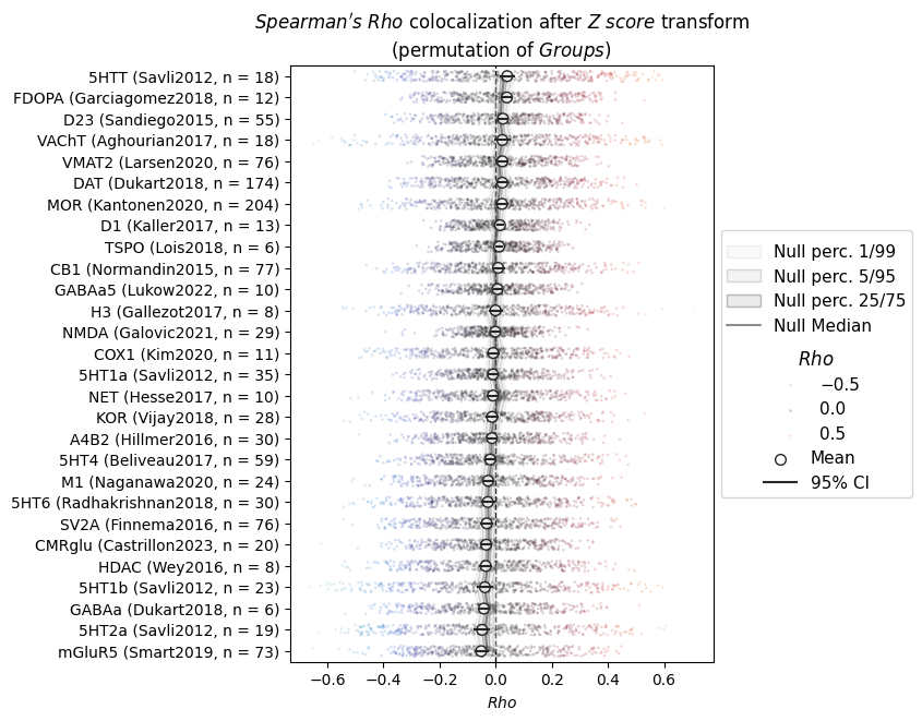
When we plot this, NiSpace will automatically detect the colocalization dataframe structure and adjust the plotting style:
[25]:
fig, ax, plot = nsp_object.plot("categorical", plot_kwargs={"sort_categories": True})
Simple X-set enrichment analysis#
Gene-set enrichment analyses (GSEA) are “an old hat” as we say in Germany (I actually have no clue, but I am quite confident that this means something else in English). They usually answer the question: “Is an input set of genes over-represented in one or more other sets of genes (e.g., markers of certain cell types or disorders) as compared to a much larger “background” gene set.
For the neuroimaging and “colocalization” space, the concept was introduced (by others first, not my idea) as a way to test if a brain map is more correlated to the brain/cortex-wide distribution of a set of genes than to other random genes. We do exactly that here. However, we call this “XSEA” as I generalized the concept to any kind of reference map dataset that is sorted into sub-categories (“sets”). Therefore, NiSpace requires the input reference data have an at least 2d-multiindex with
at least 2 levels: "map" and "set". When "mrna" is the x dataframe, subset by a collection (automatically: cell type markers), and if permute_sets=True, the function will automatically use the full gene expression dataset as background.
We use the ENIGMA example data from above.
A note on the method:#
While the original neuroimaging GSEA methods usually create a null distribution by randomly sampling gene sets from the background, NiSpace does not do that by default. Instead, it will create null maps for the input map. This is because Ben Fulcher et al. (2021) found that random set sampling can inflate false positives in sets with high coexpression (i.e., correlation) between within-set maps. As did a precourser of NiSpace,
ABAnnotate, we will use permutation of maps, which was recommended by Ben Fulcher. Note that this behavior might change with other colocalization methods; e.g., “pls” is more robust to this issue. You can pass permute_sets=True to use random set sampling instead.
[26]:
from nispace.workflows import simple_xsea

# run the analysis, plot=True will directly plot the result
colocs, p_values, q_values, nsp_object = simple_xsea(
    x="mrna",
    y=example_enigma,
    z=None, # don't control for anything on map-level
    parcellation="DesikanKilliany",
    colocalization_method="spearman", # can be any allowed method
    xsea_aggregation_method="mean",
    n_proc=-1, # number of processes, defaults to 1
    seed=42, # seed for reproducibility
    plot=False, # don't plot for now
)
INFO | 15/06/25 16:08:18 | nispace: Using integrated parcellation DesikanKilliany.
INFO | 15/06/25 16:08:18 | nispace: Loading integrated mrna dataset as X data.
INFO | 15/06/25 16:08:18 | nispace: Using collection CellTypesSilettiSuperclusters.
INFO | 15/06/25 16:08:18 | nispace: Loading mrna maps.
INFO | 15/06/25 16:08:18 | nispace: Applying collection filter from: /Users/llotter/nispace-data/reference/mrna/collection-CellTypesSilettiSuperclusters.collect.
INFO | 15/06/25 16:08:19 | nispace: Loading data parcellated with 'DesikanKilliany'
The NiSpace "mRNA" dataset is based on Allen Human Brain Atlas (AHBA) gene expression data published in Hawrylycz et al.,
2012 (https://doi.org/10.1038/nature11405). The dataset consists of mRNA expression data from postmortem brain tissue of
six donors, mapped onto MNI or fsaverage parcels using the abagen toolbox (Markello et al., 2021, https://doi.org/10.7554/eLife.72129).
The data was extracted using abagen.get_expression_data(..., lr_mirror="bidirectional"), considering parcel hemisphere and
cortical vs. subcortical location. Only genes that showed a mean donor-to-donor Spearman correlation of > 0.1 were retained.
In addition to the two publications listed above, please cite publications associated with gene set collections as appropriate.
To ensure reproducibility, note the NiSpace commit/version: 2cb3a7f5c1cea6417fe7613465a1c503f77c87c6


INFO | 15/06/25 16:08:20 | nispace: *** NiSpace.fit() - Data extraction and preparation. ***
INFO | 15/06/25 16:08:20 | nispace: Loading cortex parcellation 'DesikanKilliany' in 'MNI152NLin2009cAsym' space.
INFO | 15/06/25 16:08:20 | nispace: Loaded integrated parcellation with pre-calculated distance matrix.
INFO | 15/06/25 16:08:20 | nispace: Checking input data for 'x' (should be, e.g., PET data):
INFO | 15/06/25 16:08:20 | nispace: Input type: DataFrame, assuming parcellated data with shape (n_files/subjects/etc, n_parcels).
INFO | 15/06/25 16:08:20 | nispace: Got 'x' data for 635 x 68 parcels.
INFO | 15/06/25 16:08:20 | nispace: Checking input data for 'y' (should be, e.g., subject data):
INFO | 15/06/25 16:08:20 | nispace: Input type: Series, assuming parcellated data with shape (1, n_parcels).
INFO | 15/06/25 16:08:20 | nispace: Got 'y' data for 1 x 68 parcels.
INFO | 15/06/25 16:08:20 | nispace: Z-standardizing 'X' data.
INFO | 15/06/25 16:08:20 | nispace: *** NiSpace.colocalize() - Estimating X & Y colocalizations. ***
INFO | 15/06/25 16:08:20 | nispace: Running 'spearman' colocalization.
INFO | 15/06/25 16:08:20 | nispace: Will perform X-set enrichment analysis (XSEA).
INFO | 15/06/25 16:08:20 | nispace: Using 29 sets with between 3 and 112 samples. Aggregating within-set colocalizations with: mean.
Colocalizing (spearman, -1 proc): 100%|██████████| 1/1 [00:00<00:00, 1278.36it/s]
INFO | 15/06/25 16:08:20 | nispace: *** NiSpace.permute() - Estimate exact non-parametric p values. ***
INFO | 15/06/25 16:08:20 | nispace: Permutation of: Y maps.
INFO | 15/06/25 16:08:20 | nispace: Loading observed colocalizations (method = 'spearman').
INFO | 15/06/25 16:08:20 | nispace: Generating permuted Y maps.
INFO | 15/06/25 16:08:20 | nispace: No null maps found.
INFO | 15/06/25 16:08:20 | nispace: Generating null maps (n = 10000, null_method = 'moran').
INFO | 15/06/25 16:08:20 | nispace: Null map generation: Assuming n = 1 data vector(s) for n = 68 parcels.
INFO | 15/06/25 16:08:20 | nispace: Using provided distance matrix/matrices.
INFO | 15/06/25 16:08:20 | nispace: Generating null data separately for left and right hemisphere.
Moran null maps (-1 proc): 100%|██████████| 1/1 [00:00<00:00, 1274.09it/s]
INFO | 15/06/25 16:08:20 | nispace: Left-to-right mirroring null maps (simple mirroring).
INFO | 15/06/25 16:08:20 | nispace: Matching interhemispheric correlation. Observed correlation: 0.88
Mirroring null maps: 100%|██████████| 1/1 [00:00<00:00, 957.82it/s]
INFO | 15/06/25 16:08:20 | nispace: Null data generation finished.
INFO | 15/06/25 16:08:20 | nispace: Running X Set Enrichment Analysis (XSEA) without set permutation.
Null colocalizations (spearman, -1 proc): 100%|██████████| 10000/10000 [00:07<00:00, 1357.87it/s]
INFO | 15/06/25 16:08:28 | nispace: Calculating exact p-values (tails = {'rho': 'two'}).
INFO | 15/06/25 16:08:28 | nispace: *** NiSpace.correct_p() - Correct p values for multiple comparisons. ***
INFO | 15/06/25 16:08:28 | nispace: Returning colocalizations:
| METHOD   | XSEA | X_REDUCTION | Y_TRANSFORM |
| spearman | True | False       | False       |
INFO | 15/06/25 16:08:28 | nispace: Returning p values:
| METHOD   | PERMUTE_WHAT | XSEA | MC_METHOD | NORM  | X_REDUCTION | Y_TRANSFORM |
| spearman | ymaps        | True | None      | False | False       | False       |
INFO | 15/06/25 16:08:28 | nispace: Returning p values:
| METHOD   | PERMUTE_WHAT | XSEA | MC_METHOD | NORM  | X_REDUCTION | Y_TRANSFORM |
| spearman | ymaps        | True | fdrbh     | False | False       | False       |
The results DataFrames will have as many columns as there are sets (about 20 for cell type collections), not as there are genes:
[27]:
print("Spearman colocalizations after gene-set enrichment analysis")
display(colocs)

print("Set-permutation p-values of the colocalizations after gene-set enrichment analysis")
display(p_values)
print("As a Series, and sorted by p value:")
display(p_values.T.sort_values(by="BD"))
Spearman colocalizations after gene-set enrichment analysis
| Upper-layer IT | Deep-layer IT | Deep-layer NP | Deep-layer CT/6b | MGE interneuron | CGE interneuron | LAMP5-LHX6/Chandelier | Hippocampus CA1-3 | Hippocampus CA4 | Hippocampus DG | ... | Lower rhombic lip | Astrocyte | Oligodendrocyte | OPC | Committed OPC | Microglia | Bergmann glia | Vascular | Choroid plexus | Fibroblast | |
|---|---|---|---|---|---|---|---|---|---|---|---|---|---|---|---|---|---|---|---|---|---|
| BD | -0.280081 | -0.246911 | 0.085089 | 0.138167 | 0.006709 | -0.01691 | -0.021281 | 0.042564 | 0.090689 | 0.22303 | ... | 0.247197 | 0.090826 | 0.131521 | 0.029919 | 0.12042 | 0.137771 | 0.218324 | 0.059455 | 0.226676 | 0.001528 |
1 rows × 29 columns
Set-permutation p-values of the colocalizations after gene-set enrichment analysis
| Upper-layer IT | Deep-layer IT | Deep-layer NP | Deep-layer CT/6b | MGE interneuron | CGE interneuron | LAMP5-LHX6/Chandelier | Hippocampus CA1-3 | Hippocampus CA4 | Hippocampus DG | ... | Lower rhombic lip | Astrocyte | Oligodendrocyte | OPC | Committed OPC | Microglia | Bergmann glia | Vascular | Choroid plexus | Fibroblast | |
|---|---|---|---|---|---|---|---|---|---|---|---|---|---|---|---|---|---|---|---|---|---|
| BD | 0.0004 | 0.0028 | 0.5622 | 0.1144 | 0.8884 | 0.6612 | 0.857 | 0.5056 | 0.242 | 0.199 | ... | 0.1808 | 0.549 | 0.2318 | 0.5948 | 0.2594 | 0.5226 | 0.035 | 0.679 | 0.1352 | 0.997 |
1 rows × 29 columns
As a Series, and sorted by p value:
| BD | |
|---|---|
| Upper-layer IT | 0.0004 |
| Deep-layer IT | 0.0028 |
| Bergmann glia | 0.0350 |
| Cerebellar inhibitory | 0.0478 |
| Deep-layer CT/6b | 0.1144 |
| Choroid plexus | 0.1352 |
| Thalamic excitatory | 0.1628 |
| Lower rhombic lip | 0.1808 |
| Hippocampus DG | 0.1990 |
| MSN | 0.2268 |
| Oligodendrocyte | 0.2318 |
| Hippocampus CA4 | 0.2420 |
| Committed OPC | 0.2594 |
| Eccentric MSN | 0.3202 |
| Mammillary body | 0.4800 |
| Splatter | 0.4816 |
| Hippocampus CA1-3 | 0.5056 |
| Microglia | 0.5226 |
| Upper rhombic lip | 0.5440 |
| Astrocyte | 0.5490 |
| Deep-layer NP | 0.5622 |
| OPC | 0.5948 |
| CGE interneuron | 0.6612 |
| Vascular | 0.6790 |
| LAMP5-LHX6/Chandelier | 0.8570 |
| MGE interneuron | 0.8884 |
| Midbrain-derived inhibitory | 0.9138 |
| Amygdala excitatory | 0.9260 |
| Fibroblast | 0.9970 |
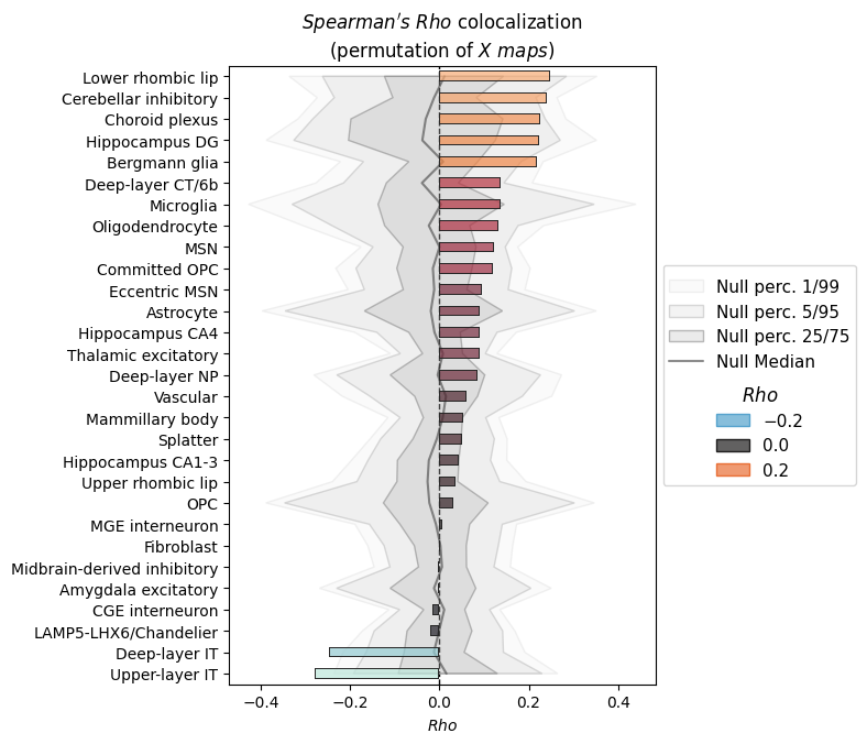
Let’s plot the result for bipolar disorder:
[28]:
fig, ax, plot = nsp_object.plot("categorical", plot_kwargs={"sort_categories": True})
INFO | 15/06/25 16:08:28 | nispace: *** NiSpace.plot() - Plot colocalization results. ***
INFO | 15/06/25 16:08:29 | nispace: Creating categorical plot for method spearman, colocalization stat rho.
[ ]: