An intro to NiSpace#
In its essence, NiSpace is a Python package for correlating brain maps with each other.
Why should we care about this, you ask?
Imports#
[1]:
# load local nispace, for testing
# COMMENT THIS OUT IF YOU RUN THIS LOCALLY AFTER INSTALLING NISPACE
import sys
sys.path.append("/Users/llotter/projects/nispace/")

# import nispace workflow function
from nispace.workflows import simple_colocalization

# import imaging functions
from nilearn.image import load_img
from nilearn.plotting import view_img
Get the T-map#
I downloaded a meta-analytically derived map automatically generated from the “pain” neuroscientific literature via NeuroQuery. This is not actually a T-map, but an effect size map. No difference for this example, though.
[2]:
# the download function is a simple function to download a file from a url and save it to a temporary directory
file_path = "neuroquery/pain.nii.gz"

# load the map into memory
effect_map = load_img(file_path)

# plot the map interactively
view_img(effect_map)
/Applications/miniforge3/envs/nsp309/lib/python3.9/site-packages/numpy/_core/fromnumeric.py:820: UserWarning: Warning: 'partition' will ignore the 'mask' of the MaskedArray.
  a.partition(kth, axis=axis, kind=kind, order=order)
[2]:
Run the analysis#
workflow function from NiSpace. Workflow functions run a complete analysis, from data loading to plotting, with a single function call.[3]:
colocalization, p_values, p_fdr_values, nispace_object = simple_colocalization(
    y={"Pain": effect_map}, # our effect map, with the dictionary we can pass a name, can also be just the effect map
    x="pet", # the PET data, here, a pre-parcellated set of PET maps is automatically downloaded
    permute_kwargs={"p_tails": "upper"}, # This tells the function to calculate right-tailed p values according to our hypothesis
    parcellation="Schaefer200", # the parcellation to use, here, Schaefer200
    seed=42, # the seed to use for the permutation analysis, for reproducibility
    n_proc=4 # number if parallel processes to use when possible
)
INFO | 15/06/25 15:58:51 | nispace: Using integrated parcellation Schaefer200.
INFO | 15/06/25 15:58:51 | nispace: Loading integrated pet dataset as X data.
INFO | 15/06/25 15:58:51 | nispace: Using collection UniqueTracers.
INFO | 15/06/25 15:58:51 | nispace: Loading pet maps.
INFO | 15/06/25 15:58:51 | nispace: Applying collection filter from: /Users/llotter/nispace-data/reference/pet/collection-UniqueTracers.collect.
INFO | 15/06/25 15:58:51 | nispace: Loading data parcellated with 'Schaefer200'
The NiSpace "PET" dataset is based on openly available nuclear imaging maps largely accessed via neuromaps
(https://neuromaps-main.readthedocs.io/). If requested in the varying original spaces and resolutions (termed "MNI152",
"fsaverageOriginal", or "fsLROriginal"), the maps are downloaded directly from the source and cached locally. If, as is highly
recommended, the maps are requested in a defined space ("MNI152NLin2009cAsym", "MNI152NLin6Asym", "fsaverage", or "fsLR"),
they are downloaded from the NiSpace-data GitHub repo (find them in `~HOME/nispace-data/reference/pet/map`).
The NiSpace-hosted MNI maps were directly registered to 2mm MNI152NLin6Asym space, and transformed to 2mm MNI152NLin2009cAsym
with a pre-estimated MNI-to-MNI transformation using SynthMorph v4 (https://martinos.org/malte/synthmorph/). The resulting maps
were masked with a liberal grey matter mask generated from the Harvard-Oxford atlas and scaled from 1e-6 to 1. The scaling was
transferred from MNI to surface maps if both were available for the same source (e.g., maps from Beliveau et al.).
The accompanying metadata table contains detailed information about tracers, source samples, original publications and data
sources, as well as the publication licenses. Every map should be cited when used. The responsibility for this lies with the user!
We additionally ask to cite:
- Markello et al., 2022 (https://doi.org/10.1038/s41592-022-01625-w)
- Hansen et al., 2022 (https://doi.org/10.1038/s41593-022-01186-3)
- Dukart et al., 2021 (https://doi.org/10.1002/hbm.25244)
- Hoffmann et al., 2024 (https://doi.org/10.1162/imag_a_00197; if NiSpace-processed maps are used)
To ensure reproducibility, note the NiSpace commit/version: 2cb3a7f5c1cea6417fe7613465a1c503f77c87c6

- target-5HT1a_tracer-way100635_n-35_dx-hc_pub-savli2012         Source: Savli2012          CC BY-NC-SA 4.0  https://doi.org/10.1016/j.neuroimage.2012.07.001
- target-5HT1b_tracer-p943_n-23_dx-hc_pub-savli2012              Source: Savli2012          CC BY-NC-SA 4.0  https://doi.org/10.1016/j.neuroimage.2012.07.001
- target-5HT2a_tracer-altanserin_n-19_dx-hc_pub-savli2012        Source: Savli2012          CC BY-NC-SA 4.0  https://doi.org/10.1016/j.neuroimage.2012.07.001
- target-5HT4_tracer-sb207145_n-59_dx-hc_pub-beliveau2017        Source: Beliveau2017       CC BY-NC-SA 4.0  https://doi.org/10.1523/JNEUROSCI.2830-16.2016
    CAVE: Processed in fsaverage space, use  volumetric maps only for subcortex! (NiSpace tables contain only fsaverage-cortical data for now.)
- target-5HT6_tracer-gsk215083_n-30_dx-hc_pub-radhakrishnan2018  Source: Radhakrishnan2018  CC BY-NC-SA 4.0  https://doi.org/10.2967/jnumed.117.206516, https://doi.org/10.1016/j.pscychresns.2019.111007
- target-5HTT_tracer-dasb_n-18_dx-hc_pub-savli2012               Source: Savli2012          CC BY-NC-SA 4.0  https://doi.org/10.1016/j.neuroimage.2012.07.001
- target-A4B2_tracer-flubatine_n-30_dx-hc_pub-hillmer2016        Source: Hillmer2016        CC BY-NC-SA 4.0  https://doi.org/10.1016/j.neuroimage.2016.07.026, https://doi.org/10.1093/ntr/ntx091
- target-CB1_tracer-omar_n-77_dx-hc_pub-normandin2015            Source: Normandin2015      CC BY-NC-SA 4.0  https://doi.org/10.1038/jcbfm.2015.46, https://doi.org/10.1016/j.bpsc.2015.09.008, https://doi.org/10.1016/j.biopsych.2015.08.021, https://doi.org/10.1111/j.1530-0277.2012.01815.x
- target-CMRglu_tracer-fdg_n-20_dx-hc_pub-castrillon2023         Source: Castrillon2023     CC BY-NC-SA 4.0  https://doi.org/10.1126/sciadv.adi7632
- target-COX1_tracer-ps13_n-11_dx-hc_pub-kim2020                 Source: Kim2020            CC0 1.0          https://doi.org/10.1007/s00259-020-04855-2, https://doi.org/10.18112/openneuro.ds004401.v1.0.1
- target-D1_tracer-sch23390_n-13_dx-hc_pub-kaller2017            Source: Kaller2017         CC BY-NC-SA 4.0  https://doi.org/10.1007/s00259-017-3645-0
- target-D23_tracer-flb457_n-55_dx-hc_pub-sandiego2015           Source: Sandiego2015       CC BY-NC-SA 4.0  https://doi.org/10.1038/jcbfm.2014.237, https://doi.org/10.1177/0271678X17737693, https://doi.org/10.1038/s41386-019-0456-y, https://doi.org/10.1001/jamapsychiatry.2014.2414, https://doi.org/10.1038/npp.2017.223
- target-DAT_tracer-fpcit_n-174_dx-hc_pub-dukart2018             Source: Dukart2018         CC BY-NC-SA 4.0  https://doi.org/10.1038/s41598-018-22444-0
    CAVE: SPECT, not PET!
- target-FDOPA_tracer-fluorodopa_n-12_dx-hc_pub-garciagomez2018  Source: Garciagomez2018    free             https://doi.org/10.33588/imagendiagnostica.901.2
- target-GABAa_tracer-flumazenil_n-6_dx-hc_pub-dukart2018        Source: Dukart2018         CC BY-NC-SA 4.0  https://doi.org/10.1038/s41598-018-22444-0
- target-GABAa5_tracer-ro154513_n-10_dx-hc_pub-lukow2022         Source: Lukow2022          CC BY 4.0        https://doi.org/10.1038/s42003-022-03268-1
- target-H3_tracer-gsk189254_n-8_dx-hc_pub-gallezot2017          Source: Gallezot2017       CC BY-NC-SA 4.0  https://doi.org/10.1177/0271678X16650697, https://doi.org/10.1038/jcbfm.2009.195
- target-HDAC_tracer-martinostat_n-8_dx-hc_pub-wey2016           Source: Wey2016            CC0 1.0          https://doi.org/10.1126/scitranslmed.aaf7551
- target-KOR_tracer-ly2795050_n-28_dx-hc_pub-vijay2018           Source: Vijay2018          CC BY-NC-SA 4.0  https://doi.org/10.1038/s41386-018-0199-1
- target-M1_tracer-lsn3172176_n-24_dx-hc_pub-naganawa2020        Source: Naganawa2020       CC BY-NC-SA 4.0  https://doi.org/10.2967/jnumed.120.246967
- target-mGluR5_tracer-abp688_n-73_dx-hc_pub-smart2019           Source: Smart2019          CC BY-NC-SA 4.0  https://doi.org/10.1007/s00259-018-4252-4
- target-MOR_tracer-carfentanil_n-204_dx-hc_pub-kantonen2020     Source: Kantonen2020       CC BY-NC-SA 4.0  https://doi.org/10.1038/mp.2017.183
- target-NET_tracer-mrb_n-10_dx-hc_pub-hesse2017                 Source: Hesse2017          CC BY-NC-SA 4.0  https://doi.org/10.1007/s00259-016-3590-3
- target-NMDA_tracer-ge179_n-29_dx-hc_pub-galovic2021            Source: Galovic2021        CC BY-NC-SA 4.0  https://doi.org/10.1001/jamaneurol.2022.4352, https://doi.org/10.1016/j.neuroimage.2021.118194, https://doi.org/10.2967/jnumed.113.130641
    CAVE: Unlike other tracers, [18F]GE-179 binds to open (active) NMDA receptors!
- target-SV2A_tracer-ucbj_n-76_dx-hc_pub-finnema2016             Source: Finnema2016        CC BY-NC-SA 4.0  https://doi.org/10.1177/0271678X17724947, https://doi.org/10.2967/jnumed.120.246967, https://doi.org/10.1177/0271678X211004312, https://doi.org/10.1186/s13195-020-00742-y, https://doi.org/10.1177/0271678X20946198, https://doi.org/10.1093/cid/ciab484, https://doi.org/10.1038/s41380-021-01184-0, https://doi.org/10.1016/j.bpsc.2015.09.008, https://doi.org/10.1111/epi.16653, https://doi.org/10.1186/s13550-020-00670-w, https://doi.org/10.1002/alz.12097, https://doi.org/10.1111/epi.14701, https://doi.org/10.1038/s41467-019-09562-7, https://doi.org/10.1001/jamaneurol.2018.1836
- target-TSPO_tracer-pbr28_n-6_dx-hc_pub-lois2018                Source: Lois2018           MIT              https://doi.org/10.1021/acschemneuro.8b00072, https://doi.org/10.5281/zenodo.1174364
- target-VAChT_tracer-feobv_n-18_dx-hc_pub-aghourian2017         Source: Aghourian2017      CC BY-NC-SA 4.0  https://doi.org/10.1038/mp.2017.183
- target-VMAT2_tracer-dtbz_n-76_dx-hc_pub-larsen2020             Source: Larsen2020         CC0 1.0          https://doi.org/10.18112/openneuro.ds002385.v1.1.0, https://doi.org/10.1038/s41467-020-14693-3

INFO | 15/06/25 15:58:51 | nispace: *** NiSpace.fit() - Data extraction and preparation. ***
INFO | 15/06/25 15:58:51 | nispace: Loading cortex parcellation 'Schaefer200' in 'MNI152NLin2009cAsym' space.
INFO | 15/06/25 15:58:51 | nispace: Loaded integrated parcellation with pre-calculated distance matrix.
INFO | 15/06/25 15:58:51 | nispace: Checking input data for 'x' (should be, e.g., PET data):
INFO | 15/06/25 15:58:51 | nispace: Input type: DataFrame, assuming parcellated data with shape (n_files/subjects/etc, n_parcels).
WARNING | 15/06/25 15:58:51 | nispace: Parcellated data contains nan values!
INFO | 15/06/25 15:58:51 | nispace: Got 'x' data for 28 x 200 parcels.
INFO | 15/06/25 15:58:51 | nispace: Checking input data for 'y' (should be, e.g., subject data):
INFO | 15/06/25 15:58:51 | nispace: Input type: dict, assuming (img_name, img) pairs for imaging data.
INFO | 15/06/25 15:58:51 | nispace: Parcellating imaging data.
INFO | 15/06/25 15:58:54 | nispace: Combined across images, 0 parcel(s) had only background intensity and were set to nan ([]).
INFO | 15/06/25 15:58:54 | nispace: Got 'y' data for 1 x 200 parcels.
INFO | 15/06/25 15:58:54 | nispace: Z-standardizing 'X' data.
INFO | 15/06/25 15:58:54 | nispace: *** NiSpace.colocalize() - Estimating X & Y colocalizations. ***
INFO | 15/06/25 15:58:54 | nispace: Running 'spearman' colocalization.
INFO | 15/06/25 15:58:57 | nispace: *** NiSpace.permute() - Estimate exact non-parametric p values. ***
INFO | 15/06/25 15:58:57 | nispace: Permutation of: X maps.
INFO | 15/06/25 15:58:57 | nispace: Loading observed colocalizations (method = 'spearman').
INFO | 15/06/25 15:58:57 | nispace: Generating permuted X maps.
INFO | 15/06/25 15:58:57 | nispace: No null maps found.
INFO | 15/06/25 15:58:57 | nispace: Generating null maps (n = 10000, null_method = 'moran').
INFO | 15/06/25 15:58:57 | nispace: Null map generation: Assuming n = 28 data vector(s) for n = 200 parcels.
INFO | 15/06/25 15:58:57 | nispace: Using provided distance matrix/matrices.
INFO | 15/06/25 15:58:57 | nispace: Generating null data separately for left and right hemisphere.
INFO | 15/06/25 15:59:00 | nispace: Left-to-right mirroring null maps (using left-to-right mapping).
INFO | 15/06/25 15:59:00 | nispace: Matching interhemispheric correlation. Observed correlation: 0.92 (mean), 0.77 - 0.98 (range)
INFO | 15/06/25 15:59:03 | nispace: Null data generation finished.
INFO | 15/06/25 15:59:03 | nispace: Z-standardizing null maps.
INFO | 15/06/25 15:59:06 | nispace: Calculating exact p-values (tails = {'rho': 'upper'}).
INFO | 15/06/25 15:59:06 | nispace: *** NiSpace.correct_p() - Correct p values for multiple comparisons. ***
INFO | 15/06/25 15:59:06 | nispace: *** NiSpace.plot() - Plot colocalization results. ***
INFO | 15/06/25 15:59:07 | nispace: Creating categorical plot for method spearman, colocalization stat rho.

INFO | 15/06/25 15:59:07 | nispace: Returning colocalizations:
| METHOD   | XSEA  | X_REDUCTION | Y_TRANSFORM |
| spearman | False | False       | False       |
INFO | 15/06/25 15:59:07 | nispace: Returning p values:
| METHOD   | PERMUTE_WHAT | XSEA  | MC_METHOD | NORM  | X_REDUCTION | Y_TRANSFORM |
| spearman | xmaps        | False | None      | False | False       | False       |
INFO | 15/06/25 15:59:07 | nispace: Returning p values:
| METHOD   | PERMUTE_WHAT | XSEA  | MC_METHOD | NORM  | X_REDUCTION | Y_TRANSFORM |
| spearman | xmaps        | False | fdrbh     | False | False       | False       |
The workflow function returns dataframes with colocalization values, p values, and FDR-corrected p values. Let’s take a look at the p values.
[4]:
# the p value dataframe contains one row for each input (y) map and one column for each reference (x) map
print("Output p values:")
display(p_values)

# we can display this a bit more nicely by transposing and sorting in ascending order
print("Sorted p values:")
p_values.T.sort_values(by="Pain")
Output p values:
| set | General | Immunity | Glutamate | GABA | ... | Serotonin | Noradrenaline/Acetylcholine | Opiods/Endocannabinoids | Histamine | ||||||||||||
|---|---|---|---|---|---|---|---|---|---|---|---|---|---|---|---|---|---|---|---|---|---|
| map | target-CMRglu_tracer-fdg_n-20_dx-hc_pub-castrillon2023 | target-SV2A_tracer-ucbj_n-76_dx-hc_pub-finnema2016 | target-HDAC_tracer-martinostat_n-8_dx-hc_pub-wey2016 | target-VMAT2_tracer-dtbz_n-76_dx-hc_pub-larsen2020 | target-TSPO_tracer-pbr28_n-6_dx-hc_pub-lois2018 | target-COX1_tracer-ps13_n-11_dx-hc_pub-kim2020 | target-mGluR5_tracer-abp688_n-73_dx-hc_pub-smart2019 | target-NMDA_tracer-ge179_n-29_dx-hc_pub-galovic2021 | target-GABAa5_tracer-ro154513_n-10_dx-hc_pub-lukow2022 | target-GABAa_tracer-flumazenil_n-6_dx-hc_pub-dukart2018 | ... | target-5HT6_tracer-gsk215083_n-30_dx-hc_pub-radhakrishnan2018 | target-5HTT_tracer-dasb_n-18_dx-hc_pub-savli2012 | target-NET_tracer-mrb_n-10_dx-hc_pub-hesse2017 | target-A4B2_tracer-flubatine_n-30_dx-hc_pub-hillmer2016 | target-M1_tracer-lsn3172176_n-24_dx-hc_pub-naganawa2020 | target-VAChT_tracer-feobv_n-18_dx-hc_pub-aghourian2017 | target-MOR_tracer-carfentanil_n-204_dx-hc_pub-kantonen2020 | target-KOR_tracer-ly2795050_n-28_dx-hc_pub-vijay2018 | target-CB1_tracer-omar_n-77_dx-hc_pub-normandin2015 | target-H3_tracer-gsk189254_n-8_dx-hc_pub-gallezot2017 |
| Pain | 0.8961 | 0.6231 | 0.9205 | 0.3875 | 0.7462 | 0.7838 | 0.1534 | 0.6478 | 0.3157 | 0.7065 | ... | 0.9088 | 0.2461 | 0.0385 | 0.4246 | 0.6982 | 0.0135 | 0.2193 | 0.0596 | 0.2327 | 0.0927 |
1 rows × 28 columns
Sorted p values:
[4]:
| Pain | ||
|---|---|---|
| set | map | |
| Noradrenaline/Acetylcholine | target-VAChT_tracer-feobv_n-18_dx-hc_pub-aghourian2017 | 0.0135 |
| target-NET_tracer-mrb_n-10_dx-hc_pub-hesse2017 | 0.0385 | |
| Opiods/Endocannabinoids | target-KOR_tracer-ly2795050_n-28_dx-hc_pub-vijay2018 | 0.0596 |
| Histamine | target-H3_tracer-gsk189254_n-8_dx-hc_pub-gallezot2017 | 0.0927 |
| Glutamate | target-mGluR5_tracer-abp688_n-73_dx-hc_pub-smart2019 | 0.1534 |
| Opiods/Endocannabinoids | target-MOR_tracer-carfentanil_n-204_dx-hc_pub-kantonen2020 | 0.2193 |
| target-CB1_tracer-omar_n-77_dx-hc_pub-normandin2015 | 0.2327 | |
| Serotonin | target-5HTT_tracer-dasb_n-18_dx-hc_pub-savli2012 | 0.2461 |
| Dopamine | target-DAT_tracer-fpcit_n-174_dx-hc_pub-dukart2018 | 0.2792 |
| GABA | target-GABAa5_tracer-ro154513_n-10_dx-hc_pub-lukow2022 | 0.3157 |
| Dopamine | target-D1_tracer-sch23390_n-13_dx-hc_pub-kaller2017 | 0.3526 |
| General | target-VMAT2_tracer-dtbz_n-76_dx-hc_pub-larsen2020 | 0.3875 |
| Serotonin | target-5HT1a_tracer-way100635_n-35_dx-hc_pub-savli2012 | 0.3910 |
| Dopamine | target-D23_tracer-flb457_n-55_dx-hc_pub-sandiego2015 | 0.4229 |
| Noradrenaline/Acetylcholine | target-A4B2_tracer-flubatine_n-30_dx-hc_pub-hillmer2016 | 0.4246 |
| Dopamine | target-FDOPA_tracer-fluorodopa_n-12_dx-hc_pub-garciagomez2018 | 0.4943 |
| General | target-SV2A_tracer-ucbj_n-76_dx-hc_pub-finnema2016 | 0.6231 |
| Serotonin | target-5HT4_tracer-sb207145_n-59_dx-hc_pub-beliveau2017 | 0.6235 |
| Glutamate | target-NMDA_tracer-ge179_n-29_dx-hc_pub-galovic2021 | 0.6478 |
| Noradrenaline/Acetylcholine | target-M1_tracer-lsn3172176_n-24_dx-hc_pub-naganawa2020 | 0.6982 |
| GABA | target-GABAa_tracer-flumazenil_n-6_dx-hc_pub-dukart2018 | 0.7065 |
| Immunity | target-TSPO_tracer-pbr28_n-6_dx-hc_pub-lois2018 | 0.7462 |
| target-COX1_tracer-ps13_n-11_dx-hc_pub-kim2020 | 0.7838 | |
| Serotonin | target-5HT2a_tracer-altanserin_n-19_dx-hc_pub-savli2012 | 0.8645 |
| General | target-CMRglu_tracer-fdg_n-20_dx-hc_pub-castrillon2023 | 0.8961 |
| Serotonin | target-5HT6_tracer-gsk215083_n-30_dx-hc_pub-radhakrishnan2018 | 0.9088 |
| General | target-HDAC_tracer-martinostat_n-8_dx-hc_pub-wey2016 | 0.9205 |
| Serotonin | target-5HT1b_tracer-p943_n-23_dx-hc_pub-savli2012 | 0.9969 |
Run the analysis in individual steps#
We will now run the same analysis in individual steps. This will give us more flexibility and transparency and might help to understand what’s happening.
Load the data#
We have loaded the effect map already. Now, we load the PET maps via nispace’s fetch_reference function. Without additional arguments, this will download and return all PET maps contained in NiSpace’s reference collection, nonlinearly aligned to defined MNI152 spaces. A long list of references will be printed automatically, like you can see in the output above.
Here, we load a predefined set of data (collection="UniqueTracers") in a specific parcellation (parcellation="Schaefer200"), which will return a dataframe of shape (n_maps, n_parcels). We suppress the reference list by setting print_references=False.
[5]:
from nispace.datasets import fetch_reference

# fetch the PET maps
pet_maps = fetch_reference("pet", parcellation="Schaefer200", collection="UniqueTracers",
                           print_references=False)

# show the dataframe
print("PET maps dataframe. Shape:", pet_maps.shape)
pet_maps.head()
INFO | 15/06/25 15:59:08 | nispace: Loading pet maps.
INFO | 15/06/25 15:59:08 | nispace: Applying collection filter from: /Users/llotter/nispace-data/reference/pet/collection-UniqueTracers.collect.
INFO | 15/06/25 15:59:08 | nispace: Loading data parcellated with 'Schaefer200'
PET maps dataframe. Shape: (28, 200)
[5]:
| hemi-L_div-Vis_lab-1 | hemi-L_div-Vis_lab-2 | hemi-L_div-Vis_lab-3 | hemi-L_div-Vis_lab-4 | hemi-L_div-Vis_lab-5 | hemi-L_div-Vis_lab-6 | hemi-L_div-Vis_lab-7 | hemi-L_div-Vis_lab-8 | hemi-L_div-Vis_lab-9 | hemi-L_div-Vis_lab-10 | ... | hemi-R_div-Default_lab-PFCm+1 | hemi-R_div-Default_lab-PFCm+2 | hemi-R_div-Default_lab-PFCm+3 | hemi-R_div-Default_lab-PFCm+4 | hemi-R_div-Default_lab-PFCm+5 | hemi-R_div-Default_lab-PFCm+6 | hemi-R_div-Default_lab-PFCm+7 | hemi-R_div-Default_lab-PCC+1 | hemi-R_div-Default_lab-PCC+2 | hemi-R_div-Default_lab-PCC+3 | ||
|---|---|---|---|---|---|---|---|---|---|---|---|---|---|---|---|---|---|---|---|---|---|---|
| set | map | |||||||||||||||||||||
| General | target-CMRglu_tracer-fdg_n-20_dx-hc_pub-castrillon2023 | 0.677147 | 0.666611 | 0.633823 | 0.712379 | 0.604150 | 0.590683 | 0.707724 | 0.684077 | 0.621863 | 0.791744 | ... | 0.694831 | 0.702473 | 0.573170 | 0.615872 | 0.563187 | 0.712010 | 0.677833 | 0.759205 | 0.874840 | 0.805161 |
| target-SV2A_tracer-ucbj_n-76_dx-hc_pub-finnema2016 | 0.651551 | 0.606582 | 0.616104 | 0.570561 | 0.536395 | 0.509607 | 0.563901 | 0.675601 | 0.618253 | 0.649548 | ... | 0.702999 | 0.730201 | 0.606722 | 0.638996 | 0.551071 | 0.654981 | 0.587189 | 0.631831 | 0.721953 | 0.708995 | |
| target-HDAC_tracer-martinostat_n-8_dx-hc_pub-wey2016 | 0.669746 | 0.698529 | 0.655808 | 0.702535 | 0.630375 | 0.546337 | 0.722179 | 0.675539 | 0.688652 | 0.739586 | ... | 0.668765 | 0.670455 | 0.567893 | 0.653233 | 0.596888 | 0.707320 | 0.600728 | 0.685817 | 0.724039 | 0.720183 | |
| target-VMAT2_tracer-dtbz_n-76_dx-hc_pub-larsen2020 | 0.037109 | 0.024958 | 0.020044 | 0.022149 | 0.012398 | 0.019778 | 0.020688 | 0.019314 | 0.012892 | 0.029316 | ... | 0.031585 | 0.028842 | 0.023119 | 0.019917 | 0.015543 | 0.018267 | 0.017619 | 0.027597 | 0.039405 | 0.031255 | |
| Immunity | target-TSPO_tracer-pbr28_n-6_dx-hc_pub-lois2018 | 0.639551 | 0.656742 | 0.672583 | 0.688357 | 0.611939 | 0.617067 | 0.632663 | 0.649550 | 0.554802 | 0.683870 | ... | 0.689789 | 0.657424 | 0.616460 | 0.652511 | 0.598470 | 0.664826 | 0.646005 | 0.631218 | 0.691273 | 0.659166 |
5 rows × 200 columns
Initialize the NiSpace instance and run the data extraction#
[6]:
from nispace.api import NiSpace

# pass the data to the NiSpace object
nsp = NiSpace(
    x=pet_maps,
    y=effect_map,
    y_labels="Pain",
    data_space="MNI152NLin6Asym",
    parcellation="Schaefer200",
)

# run the data extraction
nsp.fit()
INFO | 15/06/25 15:59:08 | nispace: *** NiSpace.fit() - Data extraction and preparation. ***
INFO | 15/06/25 15:59:08 | nispace: Loading cortex parcellation 'Schaefer200' in 'MNI152NLin2009cAsym' space.
INFO | 15/06/25 15:59:08 | nispace: Loaded integrated parcellation with pre-calculated distance matrix.
INFO | 15/06/25 15:59:08 | nispace: Checking input data for 'x' (should be, e.g., PET data):
INFO | 15/06/25 15:59:08 | nispace: Input type: DataFrame, assuming parcellated data with shape (n_files/subjects/etc, n_parcels).
WARNING | 15/06/25 15:59:08 | nispace: Parcellated data contains nan values!
INFO | 15/06/25 15:59:08 | nispace: Got 'x' data for 28 x 200 parcels.
INFO | 15/06/25 15:59:08 | nispace: Checking input data for 'y' (should be, e.g., subject data):
INFO | 15/06/25 15:59:08 | nispace: Input type: list, assuming imaging data.
INFO | 15/06/25 15:59:08 | nispace: Parcellating imaging data.
INFO | 15/06/25 15:59:08 | nispace: Combined across images, 0 parcel(s) had only background intensity and were set to nan ([]).
INFO | 15/06/25 15:59:08 | nispace: Got 'y' data for 1 x 200 parcels.
INFO | 15/06/25 15:59:08 | nispace: Z-standardizing 'X' data.
[6]:
<nispace.api.NiSpace at 0x17f950a30>
With this, we performed parcellation of the input data (the effect map). The PET maps were already passed as a dataframe with regional values.
We can take a look at the parcellated input data. Again, one row per input map, one column per parcel.
[7]:
nsp.get_y()
INFO | 15/06/25 15:59:08 | nispace: Returning Y dataframe:
| Y_TRANSFORM |
| False       |
[7]:
| hemi-L_div-Vis_lab-1 | hemi-L_div-Vis_lab-2 | hemi-L_div-Vis_lab-3 | hemi-L_div-Vis_lab-4 | hemi-L_div-Vis_lab-5 | hemi-L_div-Vis_lab-6 | hemi-L_div-Vis_lab-7 | hemi-L_div-Vis_lab-8 | hemi-L_div-Vis_lab-9 | hemi-L_div-Vis_lab-10 | ... | hemi-R_div-Default_lab-PFCm+1 | hemi-R_div-Default_lab-PFCm+2 | hemi-R_div-Default_lab-PFCm+3 | hemi-R_div-Default_lab-PFCm+4 | hemi-R_div-Default_lab-PFCm+5 | hemi-R_div-Default_lab-PFCm+6 | hemi-R_div-Default_lab-PFCm+7 | hemi-R_div-Default_lab-PCC+1 | hemi-R_div-Default_lab-PCC+2 | hemi-R_div-Default_lab-PCC+3 | |
|---|---|---|---|---|---|---|---|---|---|---|---|---|---|---|---|---|---|---|---|---|---|
| Pain | -0.436623 | -1.075635 | -0.893094 | -0.887707 | -1.139506 | -1.259002 | -1.339256 | -1.083586 | -1.389717 | -0.828569 | ... | -0.463824 | -0.154211 | 0.643321 | -0.584073 | -0.205924 | 0.174392 | 0.172215 | -0.319737 | -0.818837 | -0.344202 |
1 rows × 200 columns
Run the colocalization analysis#
We can now run the colocalization analysis. We will use the colocalize method of the NiSpace object. We use simple Spearman correlations.
[8]:
colocalization_manual = nsp.colocalize("spearman")
INFO | 15/06/25 15:59:08 | nispace: *** NiSpace.colocalize() - Estimating X & Y colocalizations. ***
INFO | 15/06/25 15:59:08 | nispace: Running 'spearman' colocalization.
colocalize method.nsp.get_colocalizations().[9]:
display(colocalization_manual)

# this should be the same as the output from the workflow function
assert (colocalization_manual.values == colocalization.values).all(), "Values are not the same"
| set | General | Immunity | Glutamate | GABA | ... | Serotonin | Noradrenaline/Acetylcholine | Opiods/Endocannabinoids | Histamine | ||||||||||||
|---|---|---|---|---|---|---|---|---|---|---|---|---|---|---|---|---|---|---|---|---|---|
| map | target-CMRglu_tracer-fdg_n-20_dx-hc_pub-castrillon2023 | target-SV2A_tracer-ucbj_n-76_dx-hc_pub-finnema2016 | target-HDAC_tracer-martinostat_n-8_dx-hc_pub-wey2016 | target-VMAT2_tracer-dtbz_n-76_dx-hc_pub-larsen2020 | target-TSPO_tracer-pbr28_n-6_dx-hc_pub-lois2018 | target-COX1_tracer-ps13_n-11_dx-hc_pub-kim2020 | target-mGluR5_tracer-abp688_n-73_dx-hc_pub-smart2019 | target-NMDA_tracer-ge179_n-29_dx-hc_pub-galovic2021 | target-GABAa5_tracer-ro154513_n-10_dx-hc_pub-lukow2022 | target-GABAa_tracer-flumazenil_n-6_dx-hc_pub-dukart2018 | ... | target-5HT6_tracer-gsk215083_n-30_dx-hc_pub-radhakrishnan2018 | target-5HTT_tracer-dasb_n-18_dx-hc_pub-savli2012 | target-NET_tracer-mrb_n-10_dx-hc_pub-hesse2017 | target-A4B2_tracer-flubatine_n-30_dx-hc_pub-hillmer2016 | target-M1_tracer-lsn3172176_n-24_dx-hc_pub-naganawa2020 | target-VAChT_tracer-feobv_n-18_dx-hc_pub-aghourian2017 | target-MOR_tracer-carfentanil_n-204_dx-hc_pub-kantonen2020 | target-KOR_tracer-ly2795050_n-28_dx-hc_pub-vijay2018 | target-CB1_tracer-omar_n-77_dx-hc_pub-normandin2015 | target-H3_tracer-gsk189254_n-8_dx-hc_pub-gallezot2017 |
| Pain | -0.162803 | -0.068091 | -0.170727 | 0.062397 | -0.134217 | -0.142131 | 0.219451 | -0.127164 | 0.111743 | -0.202272 | ... | -0.264142 | 0.176491 | 0.309315 | 0.036321 | -0.122528 | 0.435971 | 0.152101 | 0.339014 | 0.102278 | 0.304823 |
1 rows × 28 columns
Estimate p values via permutation analysis#
permute method of the NiSpace object.[10]:
p_values_manual = nsp.permute("maps", p_tails="upper", seed=42)
INFO | 15/06/25 15:59:09 | nispace: *** NiSpace.permute() - Estimate exact non-parametric p values. ***
INFO | 15/06/25 15:59:09 | nispace: Permutation of: X maps.
INFO | 15/06/25 15:59:09 | nispace: Loading observed colocalizations (method = 'spearman').
INFO | 15/06/25 15:59:09 | nispace: Generating permuted X maps.
INFO | 15/06/25 15:59:09 | nispace: No null maps found.
INFO | 15/06/25 15:59:09 | nispace: Generating null maps (n = 10000, null_method = 'moran').
INFO | 15/06/25 15:59:09 | nispace: Null map generation: Assuming n = 28 data vector(s) for n = 200 parcels.
INFO | 15/06/25 15:59:09 | nispace: Using provided distance matrix/matrices.
INFO | 15/06/25 15:59:09 | nispace: Generating null data separately for left and right hemisphere.
INFO | 15/06/25 15:59:10 | nispace: Left-to-right mirroring null maps (using left-to-right mapping).
INFO | 15/06/25 15:59:10 | nispace: Matching interhemispheric correlation. Observed correlation: 0.92 (mean), 0.77 - 0.98 (range)
INFO | 15/06/25 15:59:14 | nispace: Null data generation finished.
INFO | 15/06/25 15:59:14 | nispace: Z-standardizing null maps.
INFO | 15/06/25 15:59:19 | nispace: Calculating exact p-values (tails = {'rho': 'upper'}).
Again, we look at the results. You should have gotten the hang of it by now, right?
[11]:
display(p_values_manual)

# this should be the same as the output from the workflow function
assert (p_values_manual.values == p_values.values).all(), "Values are not the same"
| set | General | Immunity | Glutamate | GABA | ... | Serotonin | Noradrenaline/Acetylcholine | Opiods/Endocannabinoids | Histamine | ||||||||||||
|---|---|---|---|---|---|---|---|---|---|---|---|---|---|---|---|---|---|---|---|---|---|
| map | target-CMRglu_tracer-fdg_n-20_dx-hc_pub-castrillon2023 | target-SV2A_tracer-ucbj_n-76_dx-hc_pub-finnema2016 | target-HDAC_tracer-martinostat_n-8_dx-hc_pub-wey2016 | target-VMAT2_tracer-dtbz_n-76_dx-hc_pub-larsen2020 | target-TSPO_tracer-pbr28_n-6_dx-hc_pub-lois2018 | target-COX1_tracer-ps13_n-11_dx-hc_pub-kim2020 | target-mGluR5_tracer-abp688_n-73_dx-hc_pub-smart2019 | target-NMDA_tracer-ge179_n-29_dx-hc_pub-galovic2021 | target-GABAa5_tracer-ro154513_n-10_dx-hc_pub-lukow2022 | target-GABAa_tracer-flumazenil_n-6_dx-hc_pub-dukart2018 | ... | target-5HT6_tracer-gsk215083_n-30_dx-hc_pub-radhakrishnan2018 | target-5HTT_tracer-dasb_n-18_dx-hc_pub-savli2012 | target-NET_tracer-mrb_n-10_dx-hc_pub-hesse2017 | target-A4B2_tracer-flubatine_n-30_dx-hc_pub-hillmer2016 | target-M1_tracer-lsn3172176_n-24_dx-hc_pub-naganawa2020 | target-VAChT_tracer-feobv_n-18_dx-hc_pub-aghourian2017 | target-MOR_tracer-carfentanil_n-204_dx-hc_pub-kantonen2020 | target-KOR_tracer-ly2795050_n-28_dx-hc_pub-vijay2018 | target-CB1_tracer-omar_n-77_dx-hc_pub-normandin2015 | target-H3_tracer-gsk189254_n-8_dx-hc_pub-gallezot2017 |
| Pain | 0.8961 | 0.6231 | 0.9205 | 0.3875 | 0.7462 | 0.7838 | 0.1534 | 0.6478 | 0.3157 | 0.7065 | ... | 0.9088 | 0.2461 | 0.0385 | 0.4246 | 0.6982 | 0.0135 | 0.2193 | 0.0596 | 0.2327 | 0.0927 |
1 rows × 28 columns
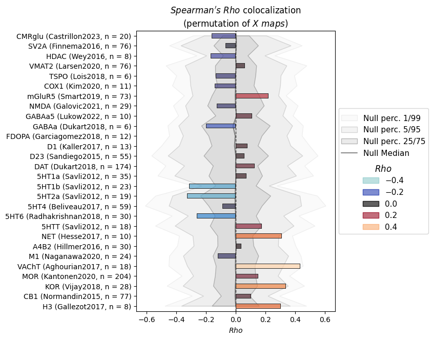
Plot the results#
There’s a plot method for the NiSpace object. It tries to find the best way to visualize the results. I admit, this it not always successful in the current state, but it’s a good starting point.
[12]:
nsp.plot()
INFO | 15/06/25 15:59:19 | nispace: *** NiSpace.plot() - Plot colocalization results. ***
INFO | 15/06/25 15:59:20 | nispace: Creating categorical plot for method spearman, colocalization stat rho.
[12]:
(<Figure size 500x710 with 1 Axes>,
 <Axes: title={'center': "$Spearman's\\ Rho$ colocalization\n(permutation of $X\\ maps$)"}, xlabel='$Rho$'>,
 <seaborn._core.plot.Plotter at 0x17ef37160>)
Save the NiSpace object#
to_pickle() method. It makes sense to use compression..pkl.pkl.gz.pkl.blosc
We recommend using .pkl.blosc for the best performance.
[13]:
import os

# save the complete nispace object
nsp.to_pickle("nispace_object.pkl.blosc")
# file size
print(f"File size: {os.path.getsize('nispace_object.pkl.blosc') / 1024**2:.2f} MB")

# save the nispace object without nulls
nsp.to_pickle("nispace_object_no_nulls.pkl.blosc", save_nulls=False)
# file size
print(f"File size when nulls are dropped: {os.path.getsize('nispace_object_no_nulls.pkl.blosc') / 1024**2:.2f} MB")
File size: 406.64 MB
File size when nulls are dropped: 3.47 MB
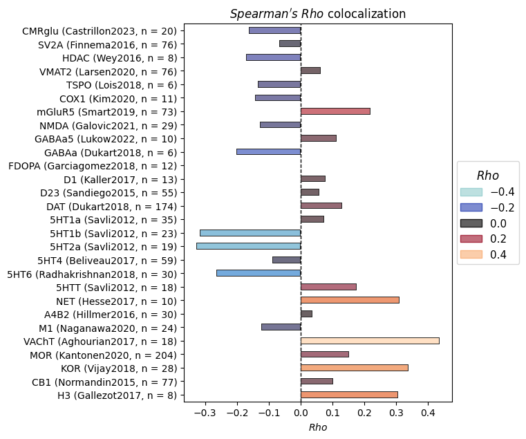
For demonstration purposes, we will now load the nispace object without nulls and try to create the plot above.
[14]:
# load the nispace object without nulls
nsp_loaded_no_nulls = NiSpace.from_pickle("nispace_object_no_nulls.pkl.blosc")
print("Reloaded nispace object:", nsp_loaded_no_nulls)

# we will get a warning if we try to plot the nispace object and the plot will not have the nulls
nsp_loaded_no_nulls.plot(plot_nulls=True)
Reloaded nispace object: <nispace.api.NiSpace object at 0x17c6334f0>
INFO | 15/06/25 15:59:22 | nispace: *** NiSpace.plot() - Plot colocalization results. ***
WARNING | 15/06/25 15:59:22 | nispace: No nulls found. Not plotting null distributions.
INFO | 15/06/25 15:59:22 | nispace: Creating categorical plot for method spearman, colocalization stat rho.
[14]:
(<Figure size 500x710 with 1 Axes>,
 <Axes: title={'center': "$Spearman's\\ Rho$ colocalization"}, xlabel='$Rho$'>,
 <seaborn._core.plot.Plotter at 0x17f2eafd0>)
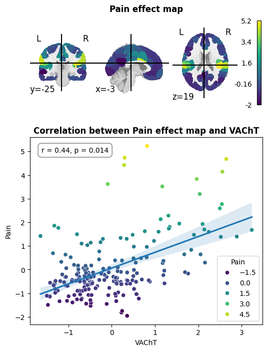
Extra: Nice correlation plot of the main result#
We will create a plot of the input data projected on a brain together with the correlation between the input map and the VAChT map, which showed the strongest colocalization.
First, load the parcellated data.
[15]:
# get the parcellated effect map
effect_map_parcellated = nsp.get_y().loc["Pain"]
display(effect_map_parcellated.head())

# get the parcellated "VAChT" PET map
k = ("Noradrenaline/Acetylcholine", "target-VAChT_tracer-feobv_n-18_dx-hc_pub-aghourian2017")
VAChT_parcellated = nsp.get_x().loc[k]
# rename to "VAChT"
VAChT_parcellated.name = "VAChT"
display(VAChT_parcellated.head())

# plot
INFO | 15/06/25 15:59:22 | nispace: Returning Y dataframe:
| Y_TRANSFORM |
| False       |
hemi-L_div-Vis_lab-1   -0.436623
hemi-L_div-Vis_lab-2   -1.075635
hemi-L_div-Vis_lab-3   -0.893094
hemi-L_div-Vis_lab-4   -0.887707
hemi-L_div-Vis_lab-5   -1.139506
Name: Pain, dtype: float32
INFO | 15/06/25 15:59:22 | nispace: Returning X dataframe:
| X_REDUCTION |
| False       |
hemi-L_div-Vis_lab-1   -0.508933
hemi-L_div-Vis_lab-2   -0.861415
hemi-L_div-Vis_lab-3   -0.726180
hemi-L_div-Vis_lab-4   -1.245316
hemi-L_div-Vis_lab-5   -1.428280
Name: VAChT, dtype: float32
Now, create the plot. Understand the code requires some knowledge of plotting in Python.
[16]:
from seaborn import regplot,scatterplot
from matplotlib import pyplot as plt
from nilearn.plotting import plot_stat_map
from nispace.utils.utils import parc_vect_to_vol

# initialize figure
fig, (ax_brain, ax_scatter) = plt.subplots(2, 1, figsize=(6, 8), gridspec_kw={"height_ratios": [1, 2]})

# plot brains, the function parc_vect_to_vol converts the parcellated vector to a 3D image given a parcellation image
ax_brain.set_title("Pain effect map", fontweight="bold")
effect_map_parcellated_img = parc_vect_to_vol(effect_map_parcellated, nsp._parc)
plot_stat_map(
    effect_map_parcellated_img,
    cmap="viridis", symmetric_cbar=False,
    axes=ax_brain
)

# plot scatter plot and regression line
ax_scatter.set_title("Correlation between Pain effect map and VAChT", fontweight="bold")
scatterplot(
    y=effect_map_parcellated, x=VAChT_parcellated,
    hue=effect_map_parcellated, palette="viridis", sizes=15,
    ax=ax_scatter
)
regplot(
    y=effect_map_parcellated, x=VAChT_parcellated,
    scatter=False,
    ax=ax_scatter
)

# plot stats results
r = colocalization_manual.loc['Pain', k]
p = p_values_manual.loc['Pain', k]
ax_scatter.annotate(
    xy=(0.05, 0.95), xycoords="axes fraction",
    text=f"r = {r:0.2f}, p = {p:0.3f}",
    ha="left", va="top",
    bbox=dict(facecolor="white", alpha=0.5, boxstyle="round,pad=0.5"),
)
[16]:
Text(0.05, 0.95, 'r = 0.44, p = 0.014')