FreeSurfer cortical thickness colocalizations in subjects with fragile X syndrome

This notebook will demonstrate how to perform a group comparison based on FreeSurfer output. For that, we will start with actual FreeSurfer output folders, to make translation to your own data as easy as possible.

We will use a small clinical sample from OpenNeuro: “Rates of cerebral protein synthesis (rCPS) in subjects with fragile X syndrome”.

Citations: https://doi.org/10.1177/0271678X221090997 and https://doi.org/10.1016/j.nbd.2020.104978.

Fragile X syndrome (FrX), as a genetic disorder, can be expected to have strong effects on cortical thickness, likely in some brain regions more than in others. These characteristics make it interesting for demonstration of colocalization analysis.

We will first download the data from OpenNeuro to a local folder. If you only want to check out how to work with cortical FreeSurfer output, and already have tabulated data for either the coarser Desikan-Killiany (“aparc”, 34 parcels per hemisphere) or the finer Destrieux parcellation (“aparc.a2009s”, 74 parcels per hemisphere), you might want to jump directly to the analysis here.

# general imports
from pathlib import Path
import numpy as np
import pandas as pd
import matplotlib.pyplot as plt


# monkey patch to make progress bars show as ASCII instead of as widgets
import tqdm.notebook
tqdm.notebook.tqdm = tqdm.tqdm
tqdm = tqdm.notebook.tqdm

# load local nispace, for testing
# COMMENT THIS OUT IF YOU RUN THIS LOCALLY AFTER INSTALLING NISPACE
import sys
sys.path.append("/Users/llotter/projects/nispace/")

Data preparation: Download a FreeSurfer sample from OpenNeuro

Although, we will use only a small part of these data, we will download the complete freesurfer/sub-{}/stats folders for each subject as we would have after we processed a dataset with FreeSurfer. It’s only table files, so a few MB overall.

This is a dictionary of the URLs of the files we want to download. Format: {"url": local_path}

from nispace.io import read_json

# get the directory of this notebook
notebook_dir = Path().absolute()

# read the URLs from the JSON file
urls = read_json(notebook_dir / "urls_ds004654-1.0.1.json")
#urls

Download all the files. If run like this, the code will download the data into: directory_of_this_notebook/ds004654-1.0.1/

from nispace.utils.utils_datasets import download

# this will be our dataset directory
dataset_dir = notebook_dir / "ds004654-1.0.1"

# iterate over the URLs and download the files
for url, fp in tqdm(urls.items(), desc="Downloading files..."):
    fp = notebook_dir / fp
    # download the file only if it does not exist already
    if not fp.exists():
        fp.parent.mkdir(parents=True, exist_ok=True)
        download(url, fp)

Downloading files...: 100%|██████████| 595/595 [00:00<00:00, 134788.60it/s]

Fetch sample data

Subject characteristics

This is a BIDS dataset, so there is a participants.tsv file that contains subject characteristics.

df_participants = pd.read_table(dataset_dir / "participants.tsv", index_col=0)

# This is what the dataframe looks like:
print("participants.tsv:")
display(df_participants.head(5))

# That's our two groups:
print("Group statistics:")
df_participants.groupby("diagnosis").describe()

participants.tsv:

	diagnosis	age	sex
participant_id
sub-HM02	HC	20	M
sub-HM03	HC	22	M
sub-HM05	HC	23	M
sub-HM06	FrX	23	M
sub-HM07	HC	20	M

Group statistics:

	age
	count	mean	std	min	25%	50%	75%	max
diagnosis
FrX	12.0	20.75	2.179449	18.0	19.0	20.5	23.0	24.0
HC	16.0	21.75	1.612452	19.0	20.0	22.0	23.0	24.0

Collect FreeSurfer data

For now, we will use standard FreeSurfer output from the cortical segmentation. The two standard parcellations are Desikan-Killiany and Destrieux. We assume that you have FreeSurfer installed on your system and accessible from the command line, so we can use the dedicated FreeSurfer command aparcstats2table to gather segmentation output across multiple subjects.

One has to run the command separately for each hemisphere and parcellation: Desikan-Killiany: “aparc” and Destrieux: “aparc.a2009s”.

import os
import subprocess

# set FreeSurfer's SUBJECTS_DIR to our datasets FreeSurfer output directory
os.environ["SUBJECTS_DIR"] = str(dataset_dir / "derivatives" / "freesurfer")

# we have to run the command separately for each hemisphere and parcellation
for hemi in ["lh", "rh"]:
    for parc in ["aparc", "aparc.a2009s"]:

        # this will be our output table file
        aparcstats_file = dataset_dir / f"stats_{parc}_{hemi}.tsv"

        # assemble the command (replace "thickness" with "volume" or "area" to get the other measures)
        cmd = [
            "aparcstats2table",
            "--subjects", " ".join(df_participants.index),
            "--hemi", hemi,
            "--parc", parc,
            "--meas", "thickness",
            "--tablefile", str(aparcstats_file)
        ]
        cmd = " ".join(cmd)
        print(cmd)
        # run the command
        subprocess.run(cmd, shell=True)

aparcstats2table --subjects sub-HM02 sub-HM03 sub-HM05 sub-HM06 sub-HM07 sub-HM08 sub-HM09 sub-HM10 sub-HM15 sub-HM16 sub-HM17 sub-HM18 sub-HM19 sub-HM21 sub-HM22 sub-HM24 sub-HM25 sub-HM28 sub-HM29 sub-HM30 sub-HM31 sub-HM32 sub-HM35 sub-HM36 sub-HM37 sub-HM38 sub-HM39 sub-HM40 --hemi lh --parc aparc --meas thickness --tablefile /Users/llotter/projects/nispace/docs/nb_examples/ds004654-1.0.1/stats_aparc_lh.tsv
SUBJECTS_DIR : /Users/llotter/projects/nispace/docs/nb_examples/ds004654-1.0.1/derivatives/freesurfer
Parsing the .stats files
Building the table..
Writing the table to /Users/llotter/projects/nispace/docs/nb_examples/ds004654-1.0.1/stats_aparc_lh.tsv
aparcstats2table --subjects sub-HM02 sub-HM03 sub-HM05 sub-HM06 sub-HM07 sub-HM08 sub-HM09 sub-HM10 sub-HM15 sub-HM16 sub-HM17 sub-HM18 sub-HM19 sub-HM21 sub-HM22 sub-HM24 sub-HM25 sub-HM28 sub-HM29 sub-HM30 sub-HM31 sub-HM32 sub-HM35 sub-HM36 sub-HM37 sub-HM38 sub-HM39 sub-HM40 --hemi lh --parc aparc.a2009s --meas thickness --tablefile /Users/llotter/projects/nispace/docs/nb_examples/ds004654-1.0.1/stats_aparc.a2009s_lh.tsv
SUBJECTS_DIR : /Users/llotter/projects/nispace/docs/nb_examples/ds004654-1.0.1/derivatives/freesurfer
Parsing the .stats files
Building the table..
Writing the table to /Users/llotter/projects/nispace/docs/nb_examples/ds004654-1.0.1/stats_aparc.a2009s_lh.tsv
aparcstats2table --subjects sub-HM02 sub-HM03 sub-HM05 sub-HM06 sub-HM07 sub-HM08 sub-HM09 sub-HM10 sub-HM15 sub-HM16 sub-HM17 sub-HM18 sub-HM19 sub-HM21 sub-HM22 sub-HM24 sub-HM25 sub-HM28 sub-HM29 sub-HM30 sub-HM31 sub-HM32 sub-HM35 sub-HM36 sub-HM37 sub-HM38 sub-HM39 sub-HM40 --hemi rh --parc aparc --meas thickness --tablefile /Users/llotter/projects/nispace/docs/nb_examples/ds004654-1.0.1/stats_aparc_rh.tsv
SUBJECTS_DIR : /Users/llotter/projects/nispace/docs/nb_examples/ds004654-1.0.1/derivatives/freesurfer
Parsing the .stats files
Building the table..
Writing the table to /Users/llotter/projects/nispace/docs/nb_examples/ds004654-1.0.1/stats_aparc_rh.tsv
aparcstats2table --subjects sub-HM02 sub-HM03 sub-HM05 sub-HM06 sub-HM07 sub-HM08 sub-HM09 sub-HM10 sub-HM15 sub-HM16 sub-HM17 sub-HM18 sub-HM19 sub-HM21 sub-HM22 sub-HM24 sub-HM25 sub-HM28 sub-HM29 sub-HM30 sub-HM31 sub-HM32 sub-HM35 sub-HM36 sub-HM37 sub-HM38 sub-HM39 sub-HM40 --hemi rh --parc aparc.a2009s --meas thickness --tablefile /Users/llotter/projects/nispace/docs/nb_examples/ds004654-1.0.1/stats_aparc.a2009s_rh.tsv
SUBJECTS_DIR : /Users/llotter/projects/nispace/docs/nb_examples/ds004654-1.0.1/derivatives/freesurfer
Parsing the .stats files
Building the table..
Writing the table to /Users/llotter/projects/nispace/docs/nb_examples/ds004654-1.0.1/stats_aparc.a2009s_rh.tsv

Get Euler number as a quality covariate

The Euler number is quite a good quality measure for structural MRI scans. FreeSurfer outputs it only via the asegstats2table command.

# this will be our output table file
asegstats_file = dataset_dir / f"stats_aseg.tsv"

# assemble the command
cmd = [
    "asegstats2table",
    "--subjects", " ".join(df_participants.index),
    "--tablefile", str(asegstats_file)
]
cmd = " ".join(cmd)
print(cmd)

# run the command
subprocess.run(cmd, shell=True)

asegstats2table --subjects sub-HM02 sub-HM03 sub-HM05 sub-HM06 sub-HM07 sub-HM08 sub-HM09 sub-HM10 sub-HM15 sub-HM16 sub-HM17 sub-HM18 sub-HM19 sub-HM21 sub-HM22 sub-HM24 sub-HM25 sub-HM28 sub-HM29 sub-HM30 sub-HM31 sub-HM32 sub-HM35 sub-HM36 sub-HM37 sub-HM38 sub-HM39 sub-HM40 --tablefile /Users/llotter/projects/nispace/docs/nb_examples/ds004654-1.0.1/stats_aseg.tsv
SUBJECTS_DIR : /Users/llotter/projects/nispace/docs/nb_examples/ds004654-1.0.1/derivatives/freesurfer
Parsing the .stats files
Building the table..
Writing the table to /Users/llotter/projects/nispace/docs/nb_examples/ds004654-1.0.1/stats_aseg.tsv

CompletedProcess(args='asegstats2table --subjects sub-HM02 sub-HM03 sub-HM05 sub-HM06 sub-HM07 sub-HM08 sub-HM09 sub-HM10 sub-HM15 sub-HM16 sub-HM17 sub-HM18 sub-HM19 sub-HM21 sub-HM22 sub-HM24 sub-HM25 sub-HM28 sub-HM29 sub-HM30 sub-HM31 sub-HM32 sub-HM35 sub-HM36 sub-HM37 sub-HM38 sub-HM39 sub-HM40 --tablefile /Users/llotter/projects/nispace/docs/nb_examples/ds004654-1.0.1/stats_aseg.tsv', returncode=0)

Load FreeSurfer stats tables

Now we load the FreeSurfer stats tables into pandas dataframes. We will combine left and right hemisphere data into one dataframe (L -> R). This is the way NiSpace works with bilateral surface data.

Desikan-Killiany parcellation

We’ll start with the Desikan-Killiany parcellation. Load left and right dataframes, drop unnecessary columns, and concatenate them.

# load left and right hemisphere data
df_desikan_lh = pd.read_table(dataset_dir / "stats_aparc_lh.tsv", index_col=0)
df_desikan_rh = pd.read_table(dataset_dir / "stats_aparc_rh.tsv", index_col=0)

# display the first 5 rows of left hemisphere
print("Desikan-Killiany left hemisphere: shape:", df_desikan_lh.shape)
display(df_desikan_lh.head(5))

# There's 3 columns we dont need for our core analysis: {lh|rh}_MeanThickness_thickness, BrainSegVolNotVent, eTIV
df_desikan_lh = df_desikan_lh.drop(columns=["lh_MeanThickness_thickness", "BrainSegVolNotVent", "eTIV"])
df_desikan_rh = df_desikan_rh.drop(columns=["rh_MeanThickness_thickness", "BrainSegVolNotVent", "eTIV"])
print("shape after dropping columns:", df_desikan_lh.shape)

# concatenate left and right hemisphere
df_desikan = pd.concat([df_desikan_lh, df_desikan_rh], axis=1)
print("Shape after concatenation:", df_desikan.shape)

Desikan-Killiany left hemisphere: shape: (28, 37)

	lh_bankssts_thickness	lh_caudalanteriorcingulate_thickness	lh_caudalmiddlefrontal_thickness	lh_cuneus_thickness	lh_entorhinal_thickness	lh_fusiform_thickness	lh_inferiorparietal_thickness	lh_inferiortemporal_thickness	lh_isthmuscingulate_thickness	lh_lateraloccipital_thickness	...	lh_superiorparietal_thickness	lh_superiortemporal_thickness	lh_supramarginal_thickness	lh_frontalpole_thickness	lh_temporalpole_thickness	lh_transversetemporal_thickness	lh_insula_thickness	lh_MeanThickness_thickness	BrainSegVolNotVent	eTIV
lh.aparc.thickness
sub-HM02	2.842	2.451	2.708	2.058	3.014	2.963	2.416	3.078	2.492	2.088	...	2.247	3.139	2.680	3.043	3.743	2.909	3.176	2.66845	1498381.0	1.852958e+06
sub-HM03	2.639	2.769	2.789	2.091	3.786	2.999	2.719	3.105	2.408	2.227	...	2.357	3.148	2.766	2.527	4.229	2.946	3.040	2.74607	1304548.0	1.609761e+06
sub-HM05	2.440	2.532	2.647	1.938	2.957	2.735	2.598	2.660	2.326	2.087	...	2.149	3.138	2.573	2.994	3.825	2.741	3.121	2.55060	1422817.0	1.525428e+06
sub-HM06	2.538	2.442	2.730	2.098	4.131	3.027	2.544	2.958	2.263	2.248	...	2.373	3.326	2.663	2.987	4.294	2.768	3.416	2.67984	1473457.0	1.950892e+06
sub-HM07	2.576	2.478	2.545	1.953	2.741	2.590	2.463	2.581	2.590	2.166	...	2.107	2.949	2.610	2.449	3.909	2.198	2.579	2.49447	1481353.0	1.856110e+06

5 rows × 37 columns

shape after dropping columns: (28, 34)
Shape after concatenation: (28, 68)

Destrieux parcellation

We’ll do the same thing for the Destrieux parcellation.

# load left and right hemisphere data
df_destrieux_lh = pd.read_table(dataset_dir / "stats_aparc.a2009s_lh.tsv", index_col=0)
df_destrieux_rh = pd.read_table(dataset_dir / "stats_aparc.a2009s_rh.tsv", index_col=0)

# display the first 5 rows of left hemisphere
print("Destrieux left hemisphere: shape:", df_destrieux_lh.shape)
display(df_destrieux_lh.head(5))

# drop the unnecessary columns
df_destrieux_lh = df_destrieux_lh.drop(columns=["lh_MeanThickness_thickness", "BrainSegVolNotVent", "eTIV"])
df_destrieux_rh = df_destrieux_rh.drop(columns=["rh_MeanThickness_thickness", "BrainSegVolNotVent", "eTIV"])
print("shape after dropping columns:", df_destrieux_lh.shape)

# concatenate left and right hemisphere
df_destrieux = pd.concat([df_destrieux_lh, df_destrieux_rh], axis=1)
print("Shape after concatenation:", df_destrieux.shape)

Destrieux left hemisphere: shape: (28, 77)

	lh_G_and_S_frontomargin_thickness	lh_G_and_S_occipital_inf_thickness	lh_G_and_S_paracentral_thickness	lh_G_and_S_subcentral_thickness	lh_G_and_S_transv_frontopol_thickness	lh_G_and_S_cingul-Ant_thickness	lh_G_and_S_cingul-Mid-Ant_thickness	lh_G_and_S_cingul-Mid-Post_thickness	lh_G_cingul-Post-dorsal_thickness	lh_G_cingul-Post-ventral_thickness	...	lh_S_precentral-inf-part_thickness	lh_S_precentral-sup-part_thickness	lh_S_suborbital_thickness	lh_S_subparietal_thickness	lh_S_temporal_inf_thickness	lh_S_temporal_sup_thickness	lh_S_temporal_transverse_thickness	lh_MeanThickness_thickness	BrainSegVolNotVent	eTIV
lh.aparc.a2009s.thickness
sub-HM02	2.669	2.045	2.278	2.818	2.824	2.771	2.922	2.680	3.208	3.248	...	2.544	2.530	2.194	2.284	2.820	2.673	2.828	2.66845	1498381.0	1.852958e+06
sub-HM03	2.564	2.214	2.569	3.028	2.472	3.122	3.057	2.928	3.142	3.013	...	2.795	2.887	2.478	2.437	2.658	2.737	2.699	2.74607	1304548.0	1.609761e+06
sub-HM05	2.247	2.427	2.347	2.733	2.791	2.751	2.916	2.743	2.778	2.696	...	2.828	2.641	2.301	2.459	2.496	2.666	2.621	2.55060	1422817.0	1.525428e+06
sub-HM06	2.508	2.372	2.502	3.089	2.841	2.806	2.725	2.787	3.341	2.398	...	2.778	2.465	2.627	2.415	2.574	2.723	2.623	2.67984	1473457.0	1.950892e+06
sub-HM07	2.323	2.329	2.557	2.778	2.428	2.649	2.808	2.602	3.128	2.865	...	2.539	2.597	2.401	2.417	2.289	2.570	2.454	2.49447	1481353.0	1.856110e+06

5 rows × 77 columns

shape after dropping columns: (28, 74)
Shape after concatenation: (28, 148)

Euler number and eTIV as covariates

Euler number is stored as “SurfaceHoles”. We will furthermore extract total intracranial volume (eTIV) data.

df_aseg = pd.read_table(dataset_dir / "stats_aseg.tsv", index_col=0)
df_aseg.head()

# We'll save them in our participants table
df_participants["euler_number"] = df_aseg["SurfaceHoles"].values
df_participants["eTIV"] = df_aseg["EstimatedTotalIntraCranialVol"].values

# lets see some descriptive statistics
df_participants.describe()

	age	euler_number	eTIV
count	28.000000	28.000000	2.800000e+01
mean	21.321429	40.000000	1.887269e+06
std	1.906200	12.719189	1.965039e+05
min	18.000000	16.000000	1.525428e+06
25%	20.000000	31.000000	1.738014e+06
50%	21.500000	39.500000	1.943034e+06
75%	23.000000	48.250000	2.012314e+06
max	24.000000	67.000000	2.260434e+06

Colocalization

Now to the main analysis. If you jumped to here, make sure that your data looks like this: (n_subjects x n_parcels)

print("For Desikan-Killiany parcellation:")
display(df_desikan.head(3))

print("For Destrieux parcellation:")
display(df_destrieux.head(3))

For Desikan-Killiany parcellation:

	lh_bankssts_thickness	lh_caudalanteriorcingulate_thickness	lh_caudalmiddlefrontal_thickness	lh_cuneus_thickness	lh_entorhinal_thickness	lh_fusiform_thickness	lh_inferiorparietal_thickness	lh_inferiortemporal_thickness	lh_isthmuscingulate_thickness	lh_lateraloccipital_thickness	...	rh_rostralanteriorcingulate_thickness	rh_rostralmiddlefrontal_thickness	rh_superiorfrontal_thickness	rh_superiorparietal_thickness	rh_superiortemporal_thickness	rh_supramarginal_thickness	rh_frontalpole_thickness	rh_temporalpole_thickness	rh_transversetemporal_thickness	rh_insula_thickness
sub-HM02	2.842	2.451	2.708	2.058	3.014	2.963	2.416	3.078	2.492	2.088	...	3.038	2.562	3.000	2.096	3.084	2.653	2.807	4.090	2.983	3.052
sub-HM03	2.639	2.769	2.789	2.091	3.786	2.999	2.719	3.105	2.408	2.227	...	3.205	2.677	3.216	2.431	3.193	2.737	3.261	4.042	2.902	3.262
sub-HM05	2.440	2.532	2.647	1.938	2.957	2.735	2.598	2.660	2.326	2.087	...	2.874	2.316	2.859	2.200	2.868	2.733	2.805	3.774	2.292	3.150

3 rows × 68 columns

For Destrieux parcellation:

	lh_G_and_S_frontomargin_thickness	lh_G_and_S_occipital_inf_thickness	lh_G_and_S_paracentral_thickness	lh_G_and_S_subcentral_thickness	lh_G_and_S_transv_frontopol_thickness	lh_G_and_S_cingul-Ant_thickness	lh_G_and_S_cingul-Mid-Ant_thickness	lh_G_and_S_cingul-Mid-Post_thickness	lh_G_cingul-Post-dorsal_thickness	lh_G_cingul-Post-ventral_thickness	...	rh_S_parieto_occipital_thickness	rh_S_pericallosal_thickness	rh_S_postcentral_thickness	rh_S_precentral-inf-part_thickness	rh_S_precentral-sup-part_thickness	rh_S_suborbital_thickness	rh_S_subparietal_thickness	rh_S_temporal_inf_thickness	rh_S_temporal_sup_thickness	rh_S_temporal_transverse_thickness
sub-HM02	2.669	2.045	2.278	2.818	2.824	2.771	2.922	2.680	3.208	3.248	...	2.337	1.559	2.201	2.677	2.833	2.248	2.697	2.667	2.820	2.889
sub-HM03	2.564	2.214	2.569	3.028	2.472	3.122	3.057	2.928	3.142	3.013	...	2.374	1.895	2.266	2.716	2.737	3.233	2.740	2.461	2.758	3.265
sub-HM05	2.247	2.427	2.347	2.733	2.791	2.751	2.916	2.743	2.778	2.696	...	2.310	1.658	2.190	2.512	2.456	2.769	2.499	2.381	2.483	2.018

3 rows × 148 columns

Fetch reference data

First, we will fetch our “reference data” for both parcellations.

In NiSpace, as “reference data”, we refer to the data that you would like to compare your sample data to. Coming from the JuSpace toolbox, this might often be a set of PET maps from different tracers.

We will go with that and load the standard set of PET maps, one per tracer for a set of unique targets. NiSpace ships both the imaging maps themselves but also pre-computed parcellated data. The latter can be fetched by passing a parcellation to the fetch_reference function.

from nispace.datasets import fetch_reference

# Desikan-Killiany
df_reference_desikan = fetch_reference(
    "pet",
    collection="UniqueTracers", # that's the default collection of PET maps
    parcellation="DesikanKilliany", # our parcellation
    print_references=True, # this will print the list of references associated with each map (true by default)
)

# Destrieux
df_reference_destrieux = fetch_reference(
    "pet",
    collection="UniqueTracers",
    parcellation="Destrieux",
    print_references=False, # we supress printing the list of references here
)

print("Shape of Desikan-Killiany reference data:", df_reference_desikan.shape)
print("Shape of Destrieux reference data:", df_reference_destrieux.shape)

INFO | 15/06/25 16:40:21 | nispace: Loading pet maps.
INFO | 15/06/25 16:40:21 | nispace: Applying collection filter from: /Users/llotter/nispace-data/reference/pet/collection-UniqueTracers.collect.
INFO | 15/06/25 16:40:21 | nispace: Loading data parcellated with 'DesikanKilliany'
The NiSpace "PET" dataset is based on openly available nuclear imaging maps largely accessed via neuromaps
(https://neuromaps-main.readthedocs.io/). If requested in the varying original spaces and resolutions (termed "MNI152",
"fsaverageOriginal", or "fsLROriginal"), the maps are downloaded directly from the source and cached locally. If, as is highly
recommended, the maps are requested in a defined space ("MNI152NLin2009cAsym", "MNI152NLin6Asym", "fsaverage", or "fsLR"),
they are downloaded from the NiSpace-data GitHub repo (find them in `~HOME/nispace-data/reference/pet/map`).
The NiSpace-hosted MNI maps were directly registered to 2mm MNI152NLin6Asym space, and transformed to 2mm MNI152NLin2009cAsym
with a pre-estimated MNI-to-MNI transformation using SynthMorph v4 (https://martinos.org/malte/synthmorph/). The resulting maps
were masked with a liberal grey matter mask generated from the Harvard-Oxford atlas and scaled from 1e-6 to 1. The scaling was
transferred from MNI to surface maps if both were available for the same source (e.g., maps from Beliveau et al.).
The accompanying metadata table contains detailed information about tracers, source samples, original publications and data
sources, as well as the publication licenses. Every map should be cited when used. The responsibility for this lies with the user!
We additionally ask to cite:
- Markello et al., 2022 (https://doi.org/10.1038/s41592-022-01625-w)
- Hansen et al., 2022 (https://doi.org/10.1038/s41593-022-01186-3)
- Dukart et al., 2021 (https://doi.org/10.1002/hbm.25244)
- Hoffmann et al., 2024 (https://doi.org/10.1162/imag_a_00197; if NiSpace-processed maps are used)
To ensure reproducibility, note the NiSpace commit/version: 2cb3a7f5c1cea6417fe7613465a1c503f77c87c6

- target-5HT1a_tracer-way100635_n-35_dx-hc_pub-savli2012         Source: Savli2012          CC BY-NC-SA 4.0  https://doi.org/10.1016/j.neuroimage.2012.07.001
- target-5HT1b_tracer-p943_n-23_dx-hc_pub-savli2012              Source: Savli2012          CC BY-NC-SA 4.0  https://doi.org/10.1016/j.neuroimage.2012.07.001
- target-5HT2a_tracer-altanserin_n-19_dx-hc_pub-savli2012        Source: Savli2012          CC BY-NC-SA 4.0  https://doi.org/10.1016/j.neuroimage.2012.07.001
- target-5HT4_tracer-sb207145_n-59_dx-hc_pub-beliveau2017        Source: Beliveau2017       CC BY-NC-SA 4.0  https://doi.org/10.1523/JNEUROSCI.2830-16.2016
    CAVE: Processed in fsaverage space, use  volumetric maps only for subcortex! (NiSpace tables contain only fsaverage-cortical data for now.)
- target-5HT6_tracer-gsk215083_n-30_dx-hc_pub-radhakrishnan2018  Source: Radhakrishnan2018  CC BY-NC-SA 4.0  https://doi.org/10.2967/jnumed.117.206516, https://doi.org/10.1016/j.pscychresns.2019.111007
- target-5HTT_tracer-dasb_n-18_dx-hc_pub-savli2012               Source: Savli2012          CC BY-NC-SA 4.0  https://doi.org/10.1016/j.neuroimage.2012.07.001
- target-A4B2_tracer-flubatine_n-30_dx-hc_pub-hillmer2016        Source: Hillmer2016        CC BY-NC-SA 4.0  https://doi.org/10.1016/j.neuroimage.2016.07.026, https://doi.org/10.1093/ntr/ntx091
- target-CB1_tracer-omar_n-77_dx-hc_pub-normandin2015            Source: Normandin2015      CC BY-NC-SA 4.0  https://doi.org/10.1038/jcbfm.2015.46, https://doi.org/10.1016/j.bpsc.2015.09.008, https://doi.org/10.1016/j.biopsych.2015.08.021, https://doi.org/10.1111/j.1530-0277.2012.01815.x
- target-CMRglu_tracer-fdg_n-20_dx-hc_pub-castrillon2023         Source: Castrillon2023     CC BY-NC-SA 4.0  https://doi.org/10.1126/sciadv.adi7632
- target-COX1_tracer-ps13_n-11_dx-hc_pub-kim2020                 Source: Kim2020            CC0 1.0          https://doi.org/10.1007/s00259-020-04855-2, https://doi.org/10.18112/openneuro.ds004401.v1.0.1
- target-D1_tracer-sch23390_n-13_dx-hc_pub-kaller2017            Source: Kaller2017         CC BY-NC-SA 4.0  https://doi.org/10.1007/s00259-017-3645-0
- target-D23_tracer-flb457_n-55_dx-hc_pub-sandiego2015           Source: Sandiego2015       CC BY-NC-SA 4.0  https://doi.org/10.1038/jcbfm.2014.237, https://doi.org/10.1177/0271678X17737693, https://doi.org/10.1038/s41386-019-0456-y, https://doi.org/10.1001/jamapsychiatry.2014.2414, https://doi.org/10.1038/npp.2017.223
- target-DAT_tracer-fpcit_n-174_dx-hc_pub-dukart2018             Source: Dukart2018         CC BY-NC-SA 4.0  https://doi.org/10.1038/s41598-018-22444-0
    CAVE: SPECT, not PET!
- target-FDOPA_tracer-fluorodopa_n-12_dx-hc_pub-garciagomez2018  Source: Garciagomez2018    free             https://doi.org/10.33588/imagendiagnostica.901.2
- target-GABAa_tracer-flumazenil_n-6_dx-hc_pub-dukart2018        Source: Dukart2018         CC BY-NC-SA 4.0  https://doi.org/10.1038/s41598-018-22444-0
- target-GABAa5_tracer-ro154513_n-10_dx-hc_pub-lukow2022         Source: Lukow2022          CC BY 4.0        https://doi.org/10.1038/s42003-022-03268-1
- target-H3_tracer-gsk189254_n-8_dx-hc_pub-gallezot2017          Source: Gallezot2017       CC BY-NC-SA 4.0  https://doi.org/10.1177/0271678X16650697, https://doi.org/10.1038/jcbfm.2009.195
- target-HDAC_tracer-martinostat_n-8_dx-hc_pub-wey2016           Source: Wey2016            CC0 1.0          https://doi.org/10.1126/scitranslmed.aaf7551
- target-KOR_tracer-ly2795050_n-28_dx-hc_pub-vijay2018           Source: Vijay2018          CC BY-NC-SA 4.0  https://doi.org/10.1038/s41386-018-0199-1
- target-M1_tracer-lsn3172176_n-24_dx-hc_pub-naganawa2020        Source: Naganawa2020       CC BY-NC-SA 4.0  https://doi.org/10.2967/jnumed.120.246967
- target-mGluR5_tracer-abp688_n-73_dx-hc_pub-smart2019           Source: Smart2019          CC BY-NC-SA 4.0  https://doi.org/10.1007/s00259-018-4252-4
- target-MOR_tracer-carfentanil_n-204_dx-hc_pub-kantonen2020     Source: Kantonen2020       CC BY-NC-SA 4.0  https://doi.org/10.1038/mp.2017.183
- target-NET_tracer-mrb_n-10_dx-hc_pub-hesse2017                 Source: Hesse2017          CC BY-NC-SA 4.0  https://doi.org/10.1007/s00259-016-3590-3
- target-NMDA_tracer-ge179_n-29_dx-hc_pub-galovic2021            Source: Galovic2021        CC BY-NC-SA 4.0  https://doi.org/10.1001/jamaneurol.2022.4352, https://doi.org/10.1016/j.neuroimage.2021.118194, https://doi.org/10.2967/jnumed.113.130641
    CAVE: Unlike other tracers, [18F]GE-179 binds to open (active) NMDA receptors!
- target-SV2A_tracer-ucbj_n-76_dx-hc_pub-finnema2016             Source: Finnema2016        CC BY-NC-SA 4.0  https://doi.org/10.1177/0271678X17724947, https://doi.org/10.2967/jnumed.120.246967, https://doi.org/10.1177/0271678X211004312, https://doi.org/10.1186/s13195-020-00742-y, https://doi.org/10.1177/0271678X20946198, https://doi.org/10.1093/cid/ciab484, https://doi.org/10.1038/s41380-021-01184-0, https://doi.org/10.1016/j.bpsc.2015.09.008, https://doi.org/10.1111/epi.16653, https://doi.org/10.1186/s13550-020-00670-w, https://doi.org/10.1002/alz.12097, https://doi.org/10.1111/epi.14701, https://doi.org/10.1038/s41467-019-09562-7, https://doi.org/10.1001/jamaneurol.2018.1836
- target-TSPO_tracer-pbr28_n-6_dx-hc_pub-lois2018                Source: Lois2018           MIT              https://doi.org/10.1021/acschemneuro.8b00072, https://doi.org/10.5281/zenodo.1174364
- target-VAChT_tracer-feobv_n-18_dx-hc_pub-aghourian2017         Source: Aghourian2017      CC BY-NC-SA 4.0  https://doi.org/10.1038/mp.2017.183
- target-VMAT2_tracer-dtbz_n-76_dx-hc_pub-larsen2020             Source: Larsen2020         CC0 1.0          https://doi.org/10.18112/openneuro.ds002385.v1.1.0, https://doi.org/10.1038/s41467-020-14693-3

INFO | 15/06/25 16:40:21 | nispace: Loading pet maps.
INFO | 15/06/25 16:40:21 | nispace: Applying collection filter from: /Users/llotter/nispace-data/reference/pet/collection-UniqueTracers.collect.
INFO | 15/06/25 16:40:21 | nispace: Loading data parcellated with 'Destrieux'
Shape of Desikan-Killiany reference data: (28, 68)
Shape of Destrieux reference data: (28, 148)

When working with parcellated data, it always makes sense to check if the parcel order aligns between different datasets. We’ll print the columns of the sample and reference data to check if they align.

Here, you can see that the columns of the sample data and reference data align, albeit having different naming schemes.

print("Columns of Desikan-Killiany sample and reference data:")
display(pd.DataFrame({"Sample": df_desikan.columns, "Reference": df_reference_desikan.columns}))

print("Columns of Destrieux sample and reference data:")
display(pd.DataFrame({"Sample": df_destrieux.columns, "Reference": df_reference_destrieux.columns}))

Columns of Desikan-Killiany sample and reference data:

	Sample	Reference
0	lh_bankssts_thickness	hemi-L_lab-bankssts
1	lh_caudalanteriorcingulate_thickness	hemi-L_lab-caudalanteriorcingulate
2	lh_caudalmiddlefrontal_thickness	hemi-L_lab-caudalmiddlefrontal
3	lh_cuneus_thickness	hemi-L_lab-cuneus
4	lh_entorhinal_thickness	hemi-L_lab-entorhinal
...	...	...
63	rh_supramarginal_thickness	hemi-R_lab-supramarginal
64	rh_frontalpole_thickness	hemi-R_lab-frontalpole
65	rh_temporalpole_thickness	hemi-R_lab-temporalpole
66	rh_transversetemporal_thickness	hemi-R_lab-transversetemporal
67	rh_insula_thickness	hemi-R_lab-insula

68 rows × 2 columns

Columns of Destrieux sample and reference data:

	Sample	Reference
0	lh_G_and_S_frontomargin_thickness	hemi-L_lab-G+and+S+frontomargin
1	lh_G_and_S_occipital_inf_thickness	hemi-L_lab-G+and+S+occipital+inf
2	lh_G_and_S_paracentral_thickness	hemi-L_lab-G+and+S+paracentral
3	lh_G_and_S_subcentral_thickness	hemi-L_lab-G+and+S+subcentral
4	lh_G_and_S_transv_frontopol_thickness	hemi-L_lab-G+and+S+transv+frontopol
...	...	...
143	rh_S_suborbital_thickness	hemi-R_lab-S+suborbital
144	rh_S_subparietal_thickness	hemi-R_lab-S+subparietal
145	rh_S_temporal_inf_thickness	hemi-R_lab-S+temporal+inf
146	rh_S_temporal_sup_thickness	hemi-R_lab-S+temporal+sup
147	rh_S_temporal_transverse_thickness	hemi-R_lab-S+temporal+transverse

148 rows × 2 columns

Check for “classical” group differences across parcels

This would be the default FreeSurfer analysis in a very easy fashion. We’ll perform a t-test for each parcel to check if there are significant differences between the two groups.

from scipy.stats import ttest_ind

# run t-test for each parcel
res_ttest = ttest_ind(
    df_desikan[df_participants.diagnosis == "FrX"],
    df_desikan[df_participants.diagnosis == "HC"],
    axis=0
)

# put the output into a dataframe
df_ttest = pd.DataFrame(
    {
        "Tvalue": res_ttest.statistic,
        "pvalue": res_ttest.pvalue,
        "df": res_ttest.df,
        "hemi": ["L" if l.startswith("lh_") else "R" for l in df_desikan.columns]
    },
    index=df_desikan.columns
)

# print the results sorted by p value
print("Results sorted by p value:")
df_ttest.sort_values("pvalue").head(5)

Results sorted by p value:

	Tvalue	pvalue	df	hemi
lh_parstriangularis_thickness	4.149075	0.000317	26.0	L
lh_rostralanteriorcingulate_thickness	3.728536	0.000945	26.0	L
lh_entorhinal_thickness	3.701004	0.001015	26.0	L
rh_middletemporal_thickness	3.354410	0.002450	26.0	R
rh_lateraloccipital_thickness	3.209261	0.003521	26.0	R

We have a simple function ready to inspect the results in a 3D viewer for one hemisphere.

We can observe a tendency towards increased cortical thickness in specific brain areas. Our colocalization analysis will now serve to find a pattern in the reference data that is most correlated with the observed pattern in the sample data. This could give us insights into potential mechanisms that could have led to the observed alteration pattern.

from nispace.plotting import view_surf

# plot
view_surf(df_ttest.loc[df_ttest.hemi == "L", "Tvalue"], parcellation="DesikanKilliany", template="fsaverage", hemi="L")

INFO | 15/06/25 16:40:21 | nispace: Loading cortex parcellation 'DesikanKilliany' in 'fsaverage' space.

Perform colocalization analysis

Finally! After all this data-wrangling, we can perform our main analysis.

Simple group comparison using the Desikan-Killiany parcellation

We’ll start with a simple group comparison based on effect size difference maps. This will do the following:

1. it will take the sample data and calculate, for each parcel, the effect size difference between the two groups

2. it will correlate the effect size difference maps with the reference data across parcels, separately for each reference map

3. it will calculate exact p values for each correlation coefficient by permuting the groups and re-running steps 1 and 2

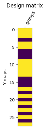
The function performs a whole workflow in one go and outputs an overview plot of the “design matrix” and the results. Minimum input are the reference and sample data, the name of the parcellation (or surface files), and a 0/1 vector indicating group memberships.

We have data for two parcellations, but we’ll start with the “simpler” Desikan-Killiany parcellation. We can expect that the results will be a bit more coarse with likely lower effect sizes for the Desikan-Killiany parcellation compared to the more fine-grained Destrieux parcellation.

from nispace.workflows import group_comparison

# we will pass this as the "design" argument. in the simplest case, this is a 0/1 vector indicating group memberships
design = df_participants.diagnosis.map({"FrX": 0, "HC": 1})
display(design.head(5))

# instead of only the groups vector, we can also pass covariates as in a GLM's design matrix
# we will not do that here, as it will not have much effects in the small sample
# only the variable "groups" is required, every other covariate is optional and will be regressed out
# of each parcel's data across subjects before the colocalization analysis
# we can do paired analyses by passing a "subjects" + the "groups" vector (then, e.g., timepoints).
# design = pd.DataFrame({
#     "groups": df_participants.diagnosis.map({"FrX": 0, "HC": 1}),
#     "age": df_participants.age,
#     "euler_number": df_participants.euler_number,
#     "eTIV": df_participants.eTIV
# })
# display(design.head(5))

# run
colocs, pvalues, qvalues, nsp_object = group_comparison(
    y=df_desikan, # sample data
    x=df_reference_desikan, # reference data
    parcellation="DesikanKilliany", # parcellation
    design=design, # group membership
    comparison_method="hedges(a,b)", # effect size difference
    colocalization_method="spearman", # spearman correlation betw. each x and y
    n_perm=10000, # number of permutations for exact p values
    n_proc=-1, # number of cores to use (-1 = all available)
    verbose=True,
)

participant_id
sub-HM02    1
sub-HM03    1
sub-HM05    1
sub-HM06    0
sub-HM07    1
Name: diagnosis, dtype: int64

INFO | 15/06/25 16:40:22 | nispace: Using integrated parcellation DesikanKilliany.
INFO | 15/06/25 16:40:22 | nispace: *** NiSpace.fit() - Data extraction and preparation. ***
INFO | 15/06/25 16:40:22 | nispace: Loading cortex parcellation 'DesikanKilliany' in 'MNI152NLin2009cAsym' space.
INFO | 15/06/25 16:40:22 | nispace: Loaded integrated parcellation with pre-calculated distance matrix.
INFO | 15/06/25 16:40:22 | nispace: Checking input data for 'x' (should be, e.g., PET data):
INFO | 15/06/25 16:40:22 | nispace: Input type: DataFrame, assuming parcellated data with shape (n_files/subjects/etc, n_parcels).
WARNING | 15/06/25 16:40:22 | nispace: Parcellated data contains nan values!
INFO | 15/06/25 16:40:22 | nispace: Got 'x' data for 28 x 68 parcels.
INFO | 15/06/25 16:40:22 | nispace: Checking input data for 'y' (should be, e.g., subject data):
INFO | 15/06/25 16:40:22 | nispace: Input type: DataFrame, assuming parcellated data with shape (n_files/subjects/etc, n_parcels).
INFO | 15/06/25 16:40:22 | nispace: Got 'y' data for 28 x 68 parcels.
INFO | 15/06/25 16:40:22 | nispace: Z-standardizing 'X' data.
INFO | 15/06/25 16:40:22 | nispace: 1d array provided for design. Assuming this to be dummy-coded groups!
INFO | 15/06/25 16:40:22 | nispace: Design matrix of shape (28, 1). Assuming 28 subjects/maps.

INFO | 15/06/25 16:40:22 | nispace: *** NiSpace.transform_y() - Y transformation and comparison. ***
INFO | 15/06/25 16:40:22 | nispace: Groups/sessions vector provided, ensuring dummy-coding.
INFO | 15/06/25 16:40:22 | nispace: Applying Y transform 'hedges(a,b)'.
INFO | 15/06/25 16:40:22 | nispace: *** NiSpace.colocalize() - Estimating X & Y colocalizations. ***
INFO | 15/06/25 16:40:22 | nispace: Running 'spearman' colocalization with 'hedges(a,b)' transform.

Colocalizing (spearman, -1 proc): 100%|██████████| 1/1 [00:00<00:00, 84.29it/s]

INFO | 15/06/25 16:40:26 | nispace: *** NiSpace.permute() - Estimate exact non-parametric p values. ***
INFO | 15/06/25 16:40:26 | nispace: Permutation of: Y groups.
INFO | 15/06/25 16:40:26 | nispace: Loading transformed Y data, transform = 'hedges(a,b)'.
INFO | 15/06/25 16:40:26 | nispace: Will calculate p values for mean calculation across Y maps. Set 'p_from_average_y_coloc' = False to change this behavior.
INFO | 15/06/25 16:40:26 | nispace: Loading observed colocalizations (method = 'spearman').
INFO | 15/06/25 16:40:26 | nispace: Generating permuted Y groups.
INFO | 15/06/25 16:40:26 | nispace: Permuting groups/sessions vector, strategy: unpaired, proportional.

Permuting groups (-1 proc): 100%|██████████| 10000/10000 [00:00<00:00, 107322.53it/s]
Null transformations (spearman, -1 proc): 100%|██████████| 10000/10000 [00:01<00:00, 8861.95it/s]
Null colocalizations (spearman, -1 proc): 100%|██████████| 10000/10000 [00:01<00:00, 6373.81it/s]

INFO | 15/06/25 16:40:32 | nispace: Calculating exact p-values (tails = {'rho': 'two'}).
INFO | 15/06/25 16:40:32 | nispace: *** NiSpace.correct_p() - Correct p values for multiple comparisons. ***
INFO | 15/06/25 16:40:32 | nispace: *** NiSpace.plot() - Plot colocalization results. ***
INFO | 15/06/25 16:40:33 | nispace: Creating categorical plot for method spearman, colocalization stat rho.

INFO | 15/06/25 16:40:33 | nispace: Returning colocalizations:
| METHOD   | XSEA  | X_REDUCTION | Y_TRANSFORM |
| spearman | False | False       | hedges(a,b) | 
INFO | 15/06/25 16:40:33 | nispace: Returning p values:
| METHOD   | PERMUTE_WHAT | XSEA  | MC_METHOD | NORM  | X_REDUCTION | Y_TRANSFORM |
| spearman | groups       | False | None      | False | False       | hedges(a,b) | 
INFO | 15/06/25 16:40:33 | nispace: Returning p values:
| METHOD   | PERMUTE_WHAT | XSEA  | MC_METHOD | NORM  | X_REDUCTION | Y_TRANSFORM |
| spearman | groups       | False | fdrbh     | False | False       | hedges(a,b) | 

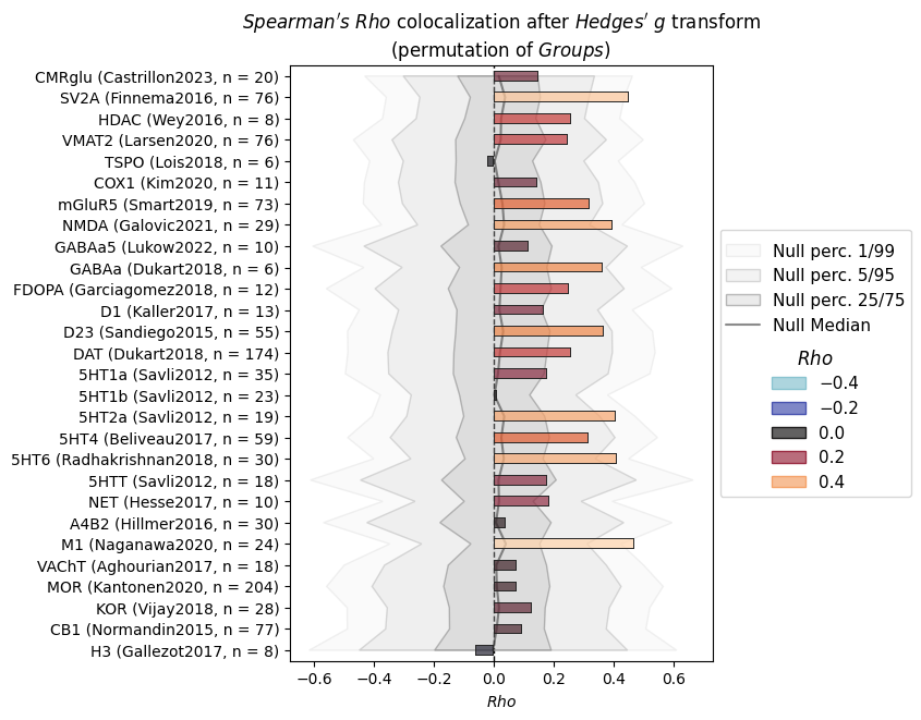
The plot (null distributions in gray) shows that there are some borderline significant results but the effects are not too strong. As said above, we can expect the results to be stronger with the more fine-grained Destrieux parcellation.

Here’s the top 5 results (FDR-corrected) of the Desikan-Killiany results (not significant at FDR=0.05):

qvalues.T["mean"].sort_values().head(5)

set                          map
General                      target-SV2A_tracer-ucbj_n-76_dx-hc_pub-finnema2016               0.22960
Noradrenaline/Acetylcholine  target-M1_tracer-lsn3172176_n-24_dx-hc_pub-naganawa2020          0.22960
Glutamate                    target-NMDA_tracer-ge179_n-29_dx-hc_pub-galovic2021              0.25200
Serotonin                    target-5HT6_tracer-gsk215083_n-30_dx-hc_pub-radhakrishnan2018    0.25200
                             target-5HT2a_tracer-altanserin_n-19_dx-hc_pub-savli2012          0.27888
Name: mean, dtype: float32

The outputs of the workflow function are:

• colocs: the correlation coefficients between the effect size maps and the reference data across parcels

• pvalues: the p values for each correlation coefficient

• qvalues: the FDR-corrected p values for each correlation coefficient

• nsp_object: the NiSpace object, which contains the results and can be used for further analyses

We will print the first three dataframes:

display("Colocalization:", colocs)
display("p values:", pvalues)
display("q values:", qvalues)

'Colocalization:'

set	General				Immunity		Glutamate		GABA		...	Serotonin		Noradrenaline/Acetylcholine				Opiods/Endocannabinoids			Histamine
map	target-CMRglu_tracer-fdg_n-20_dx-hc_pub-castrillon2023	target-SV2A_tracer-ucbj_n-76_dx-hc_pub-finnema2016	target-HDAC_tracer-martinostat_n-8_dx-hc_pub-wey2016	target-VMAT2_tracer-dtbz_n-76_dx-hc_pub-larsen2020	target-TSPO_tracer-pbr28_n-6_dx-hc_pub-lois2018	target-COX1_tracer-ps13_n-11_dx-hc_pub-kim2020	target-mGluR5_tracer-abp688_n-73_dx-hc_pub-smart2019	target-NMDA_tracer-ge179_n-29_dx-hc_pub-galovic2021	target-GABAa5_tracer-ro154513_n-10_dx-hc_pub-lukow2022	target-GABAa_tracer-flumazenil_n-6_dx-hc_pub-dukart2018	...	target-5HT6_tracer-gsk215083_n-30_dx-hc_pub-radhakrishnan2018	target-5HTT_tracer-dasb_n-18_dx-hc_pub-savli2012	target-NET_tracer-mrb_n-10_dx-hc_pub-hesse2017	target-A4B2_tracer-flubatine_n-30_dx-hc_pub-hillmer2016	target-M1_tracer-lsn3172176_n-24_dx-hc_pub-naganawa2020	target-VAChT_tracer-feobv_n-18_dx-hc_pub-aghourian2017	target-MOR_tracer-carfentanil_n-204_dx-hc_pub-kantonen2020	target-KOR_tracer-ly2795050_n-28_dx-hc_pub-vijay2018	target-CB1_tracer-omar_n-77_dx-hc_pub-normandin2015	target-H3_tracer-gsk189254_n-8_dx-hc_pub-gallezot2017
hedges	0.147879	0.45021	0.257929	0.245451	-0.023862	0.145149	0.317631	0.396057	0.113513	0.364055	...	0.411043	0.17885	0.185122	0.040447	0.468654	0.076186	0.074304	0.126874	0.093026	-0.061343

1 rows × 28 columns

'p values:'

set	General				Immunity		Glutamate		GABA		...	Serotonin		Noradrenaline/Acetylcholine				Opiods/Endocannabinoids			Histamine
map	target-CMRglu_tracer-fdg_n-20_dx-hc_pub-castrillon2023	target-SV2A_tracer-ucbj_n-76_dx-hc_pub-finnema2016	target-HDAC_tracer-martinostat_n-8_dx-hc_pub-wey2016	target-VMAT2_tracer-dtbz_n-76_dx-hc_pub-larsen2020	target-TSPO_tracer-pbr28_n-6_dx-hc_pub-lois2018	target-COX1_tracer-ps13_n-11_dx-hc_pub-kim2020	target-mGluR5_tracer-abp688_n-73_dx-hc_pub-smart2019	target-NMDA_tracer-ge179_n-29_dx-hc_pub-galovic2021	target-GABAa5_tracer-ro154513_n-10_dx-hc_pub-lukow2022	target-GABAa_tracer-flumazenil_n-6_dx-hc_pub-dukart2018	...	target-5HT6_tracer-gsk215083_n-30_dx-hc_pub-radhakrishnan2018	target-5HTT_tracer-dasb_n-18_dx-hc_pub-savli2012	target-NET_tracer-mrb_n-10_dx-hc_pub-hesse2017	target-A4B2_tracer-flubatine_n-30_dx-hc_pub-hillmer2016	target-M1_tracer-lsn3172176_n-24_dx-hc_pub-naganawa2020	target-VAChT_tracer-feobv_n-18_dx-hc_pub-aghourian2017	target-MOR_tracer-carfentanil_n-204_dx-hc_pub-kantonen2020	target-KOR_tracer-ly2795050_n-28_dx-hc_pub-vijay2018	target-CB1_tracer-omar_n-77_dx-hc_pub-normandin2015	target-H3_tracer-gsk189254_n-8_dx-hc_pub-gallezot2017
mean	0.496	0.0164	0.1684	0.3216	0.897	0.5398	0.1592	0.0346	0.7084	0.1138	...	0.036	0.5642	0.3138	0.902	0.0082	0.7904	0.812	0.6318	0.7252	0.8368

1 rows × 28 columns

'q values:'

set	General				Immunity		Glutamate		GABA		...	Serotonin		Noradrenaline/Acetylcholine				Opiods/Endocannabinoids			Histamine
map	target-CMRglu_tracer-fdg_n-20_dx-hc_pub-castrillon2023	target-SV2A_tracer-ucbj_n-76_dx-hc_pub-finnema2016	target-HDAC_tracer-martinostat_n-8_dx-hc_pub-wey2016	target-VMAT2_tracer-dtbz_n-76_dx-hc_pub-larsen2020	target-TSPO_tracer-pbr28_n-6_dx-hc_pub-lois2018	target-COX1_tracer-ps13_n-11_dx-hc_pub-kim2020	target-mGluR5_tracer-abp688_n-73_dx-hc_pub-smart2019	target-NMDA_tracer-ge179_n-29_dx-hc_pub-galovic2021	target-GABAa5_tracer-ro154513_n-10_dx-hc_pub-lukow2022	target-GABAa_tracer-flumazenil_n-6_dx-hc_pub-dukart2018	...	target-5HT6_tracer-gsk215083_n-30_dx-hc_pub-radhakrishnan2018	target-5HTT_tracer-dasb_n-18_dx-hc_pub-savli2012	target-NET_tracer-mrb_n-10_dx-hc_pub-hesse2017	target-A4B2_tracer-flubatine_n-30_dx-hc_pub-hillmer2016	target-M1_tracer-lsn3172176_n-24_dx-hc_pub-naganawa2020	target-VAChT_tracer-feobv_n-18_dx-hc_pub-aghourian2017	target-MOR_tracer-carfentanil_n-204_dx-hc_pub-kantonen2020	target-KOR_tracer-ly2795050_n-28_dx-hc_pub-vijay2018	target-CB1_tracer-omar_n-77_dx-hc_pub-normandin2015	target-H3_tracer-gsk189254_n-8_dx-hc_pub-gallezot2017
mean	0.816941	0.2296	0.523911	0.692677	0.935407	0.831453	0.523911	0.252	0.922982	0.523911	...	0.252	0.831453	0.692677	0.935407	0.2296	0.935407	0.935407	0.88452	0.922982	0.935407

1 rows × 28 columns

Simple group comparison using the Destrieux parcellation

Let’s see how the results look like with the more fine-grained Destrieux parcellation.

# rerun with Destrieux parcellation, suppress output and design matrix plotting
colocs_es, pvalues_es, qvalues_es, nsp_object_es = group_comparison(
    y=df_destrieux, # sample data
    x=df_reference_destrieux, # reference data
    parcellation="Destrieux", # parcellation
    design=design, # group membership or "design matrix"
    comparison_method="hedges(a,b)", # effect size difference
    colocalization_method="spearman", # spearman correlation betw. each x and y
    n_perm=10000, # number of permutations for exact p values
    n_proc=-1, # number of cores to use (-1 = all available)
    verbose=False,
    plot_design=False,
)

INFO | 15/06/25 16:40:33 | nispace: Loading cortex parcellation 'Destrieux' in 'MNI152NLin2009cAsym' space.
INFO | 15/06/25 16:40:33 | nispace: Loaded integrated parcellation with pre-calculated distance matrix.
INFO | 15/06/25 16:40:33 | nispace: Checking input data for 'x' (should be, e.g., PET data):

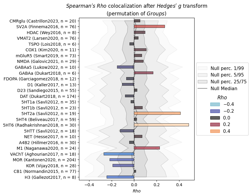
There we go! The results pattern is expectedly similar, but with stronger effects and higher specificity. We find clear positive correlations between cortical thickness alteration patterns in fragile X syndrome and 5HT2a, 5HT6, GABAa and M1 receptors, as well as synaptic density (SV2A) and transcriptomic activity (HDAC).

The positive correlation here means that areas with increased cortical thickness in fragile X syndrome versus controls are those with the highest density of the mentioned molecules in “healthy” brains.

Let’s take a short look at the FDR-corrected p values across the two parcellations:

pvalues_es.T["mean"].sort_values().head(6)

set                          map
Serotonin                    target-5HT6_tracer-gsk215083_n-30_dx-hc_pub-radhakrishnan2018    0.0001
                             target-5HT2a_tracer-altanserin_n-19_dx-hc_pub-savli2012          0.0048
General                      target-SV2A_tracer-ucbj_n-76_dx-hc_pub-finnema2016               0.0224
Noradrenaline/Acetylcholine  target-M1_tracer-lsn3172176_n-24_dx-hc_pub-naganawa2020          0.0472
                             target-VAChT_tracer-feobv_n-18_dx-hc_pub-aghourian2017           0.1286
Histamine                    target-H3_tracer-gsk189254_n-8_dx-hc_pub-gallezot2017            0.2382
Name: mean, dtype: float32

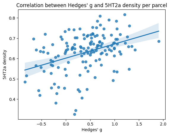
And this would be what the correlation itself looks like for a single reference map:

import matplotlib.pyplot as plt
from seaborn import regplot

regplot(
    x=nsp_object_es.get_y(Y_transform="hedges(a,b)").loc["hedges"],
    y=df_reference_destrieux.loc[("Serotonin", "target-5HT2a_tracer-altanserin_n-19_dx-hc_pub-savli2012")],
)
plt.xlabel("Hedges' g")
plt.ylabel("5HT2a density")
plt.title("Correlation between Hedges' g and 5HT2a density per parcel")

Text(0.5, 1.0, "Correlation between Hedges' g and 5HT2a density per parcel")

Advanced analyses: Group comparison using single-subject zscores

This is the standard workflow introduced with the JuSpace toolbox. The difference to above is that we do not calculate a single group-level effect size map, but instead we will calculate a z-score map for each subject as in ( case_subject - mean(control_subjects) ) / sd(control_subjects). The automatically generated plots will show individual-level values as dots instead of the bars seen above.

The results should be similar, but we will have single-subject correlation coefficients, which is quite useful for follow-up analyses. I.e., we could check whether the individual alignment with a given PET map is associated with a clinical variable of interest. This analysis will take a bit longer in larger samples because of more necessary computations.

colocs_zscore, pvalues_zscore, qvalues_zscore, nsp_object_zscore = group_comparison(
    y=df_destrieux, # sample data
    x=df_reference_destrieux, # reference data
    parcellation="Destrieux", # parcellation
    design=design, # group membership
    comparison_method="zscore(a,b)",
    colocalization_method="spearman", # spearman correlation betw. each x and y
    n_perm=10000, # number of permutations for exact p values
    n_proc=-1, # number of cores to use (-1 = all available)
    verbose=False,
    plot_design=False,
)

INFO | 15/06/25 16:40:37 | nispace: Loading cortex parcellation 'Destrieux' in 'MNI152NLin2009cAsym' space.
INFO | 15/06/25 16:40:37 | nispace: Loaded integrated parcellation with pre-calculated distance matrix.
INFO | 15/06/25 16:40:37 | nispace: Checking input data for 'x' (should be, e.g., PET data):

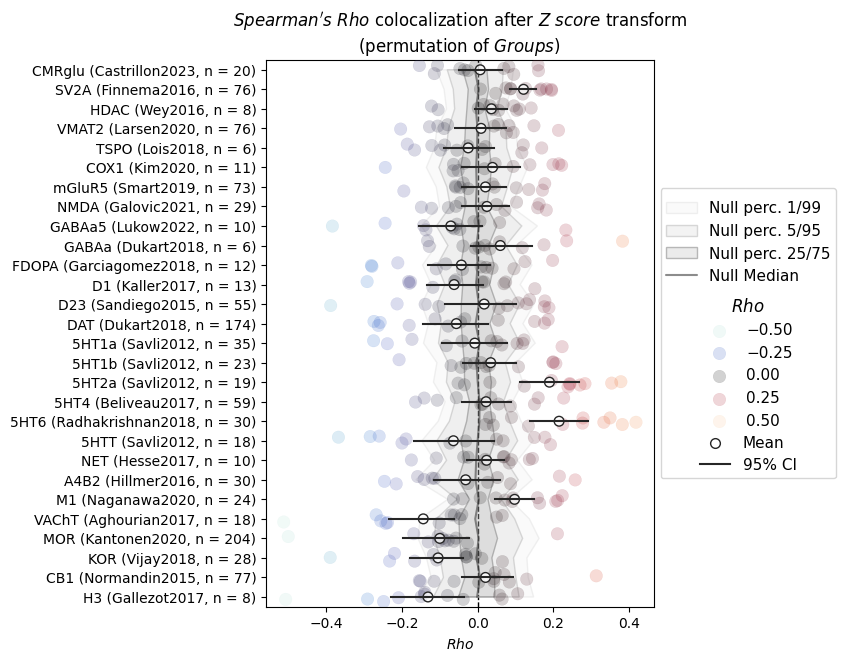
As we now have single-subject correlation coefficients for all FrX subjects, the resulting colocalization dataframe will have one row for each subject. P values, however, are by default calculated for the mean of the sample, so they will still have one row across all subjects.

display("Colocalization:", colocs_zscore.head(3))
display("P values:", pvalues_zscore)

'Colocalization:'

set	General				Immunity		Glutamate		GABA		...	Serotonin		Noradrenaline/Acetylcholine				Opiods/Endocannabinoids			Histamine
map	target-CMRglu_tracer-fdg_n-20_dx-hc_pub-castrillon2023	target-SV2A_tracer-ucbj_n-76_dx-hc_pub-finnema2016	target-HDAC_tracer-martinostat_n-8_dx-hc_pub-wey2016	target-VMAT2_tracer-dtbz_n-76_dx-hc_pub-larsen2020	target-TSPO_tracer-pbr28_n-6_dx-hc_pub-lois2018	target-COX1_tracer-ps13_n-11_dx-hc_pub-kim2020	target-mGluR5_tracer-abp688_n-73_dx-hc_pub-smart2019	target-NMDA_tracer-ge179_n-29_dx-hc_pub-galovic2021	target-GABAa5_tracer-ro154513_n-10_dx-hc_pub-lukow2022	target-GABAa_tracer-flumazenil_n-6_dx-hc_pub-dukart2018	...	target-5HT6_tracer-gsk215083_n-30_dx-hc_pub-radhakrishnan2018	target-5HTT_tracer-dasb_n-18_dx-hc_pub-savli2012	target-NET_tracer-mrb_n-10_dx-hc_pub-hesse2017	target-A4B2_tracer-flubatine_n-30_dx-hc_pub-hillmer2016	target-M1_tracer-lsn3172176_n-24_dx-hc_pub-naganawa2020	target-VAChT_tracer-feobv_n-18_dx-hc_pub-aghourian2017	target-MOR_tracer-carfentanil_n-204_dx-hc_pub-kantonen2020	target-KOR_tracer-ly2795050_n-28_dx-hc_pub-vijay2018	target-CB1_tracer-omar_n-77_dx-hc_pub-normandin2015	target-H3_tracer-gsk189254_n-8_dx-hc_pub-gallezot2017
sub-HM06	-0.153929	0.007294	-0.104420	0.076167	0.020851	-0.035747	-0.046130	-0.057443	0.058151	-0.127871	...	0.020743	0.149822	0.089360	-0.246324	-0.040208	-0.061688	-0.104471	-0.232777	0.083851	-0.140744
sub-HM09	0.161004	0.168028	0.066939	0.043035	-0.121139	0.018174	0.135101	0.102845	-0.136747	0.032122	...	0.031551	-0.199951	-0.036917	0.257904	0.071968	0.049628	-0.092817	-0.030405	-0.151537	0.105929
sub-HM10	0.159378	0.126809	0.103099	-0.203596	-0.166683	0.046041	0.039254	-0.121843	-0.244572	-0.132404	...	0.041281	-0.367951	0.020064	0.216137	-0.063887	-0.069980	-0.026912	-0.029424	-0.115149	0.057532

3 rows × 28 columns

'P values:'

set	General				Immunity		Glutamate		GABA		...	Serotonin		Noradrenaline/Acetylcholine				Opiods/Endocannabinoids			Histamine
map	target-CMRglu_tracer-fdg_n-20_dx-hc_pub-castrillon2023	target-SV2A_tracer-ucbj_n-76_dx-hc_pub-finnema2016	target-HDAC_tracer-martinostat_n-8_dx-hc_pub-wey2016	target-VMAT2_tracer-dtbz_n-76_dx-hc_pub-larsen2020	target-TSPO_tracer-pbr28_n-6_dx-hc_pub-lois2018	target-COX1_tracer-ps13_n-11_dx-hc_pub-kim2020	target-mGluR5_tracer-abp688_n-73_dx-hc_pub-smart2019	target-NMDA_tracer-ge179_n-29_dx-hc_pub-galovic2021	target-GABAa5_tracer-ro154513_n-10_dx-hc_pub-lukow2022	target-GABAa_tracer-flumazenil_n-6_dx-hc_pub-dukart2018	...	target-5HT6_tracer-gsk215083_n-30_dx-hc_pub-radhakrishnan2018	target-5HTT_tracer-dasb_n-18_dx-hc_pub-savli2012	target-NET_tracer-mrb_n-10_dx-hc_pub-hesse2017	target-A4B2_tracer-flubatine_n-30_dx-hc_pub-hillmer2016	target-M1_tracer-lsn3172176_n-24_dx-hc_pub-naganawa2020	target-VAChT_tracer-feobv_n-18_dx-hc_pub-aghourian2017	target-MOR_tracer-carfentanil_n-204_dx-hc_pub-kantonen2020	target-KOR_tracer-ly2795050_n-28_dx-hc_pub-vijay2018	target-CB1_tracer-omar_n-77_dx-hc_pub-normandin2015	target-H3_tracer-gsk189254_n-8_dx-hc_pub-gallezot2017
mean	0.7696	0.0008	0.2396	0.845	0.6316	0.4728	0.6528	0.4926	0.2874	0.1896	...	0.0001	0.3292	0.5584	0.713	0.0072	0.03	0.1538	0.0816	0.7972	0.0594

1 rows × 28 columns

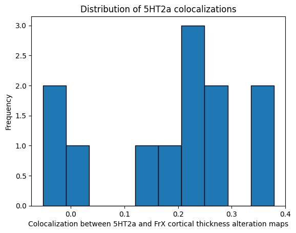
Post-hoc analyses

As mentioned above, if using the “zscore” group comparison method, we can perform post-hoc analyses on the single-subject correlation coefficients. This just serves to demonstrate how to work with the colocalization results.

In our small sample, we will not find much interesting.

# colocalizations for 5HT2a
colocs_5HT2a = colocs_zscore.loc[:, ("Serotonin", "target-5HT2a_tracer-altanserin_n-19_dx-hc_pub-savli2012")]

# show the distributions of these values
colocs_5HT2a.plot.hist(legend=False, title="Distribution of 5HT2a colocalizations", edgecolor="k")
plt.xlabel("Colocalization between 5HT2a and FrX cortical thickness alteration maps")
plt.show()

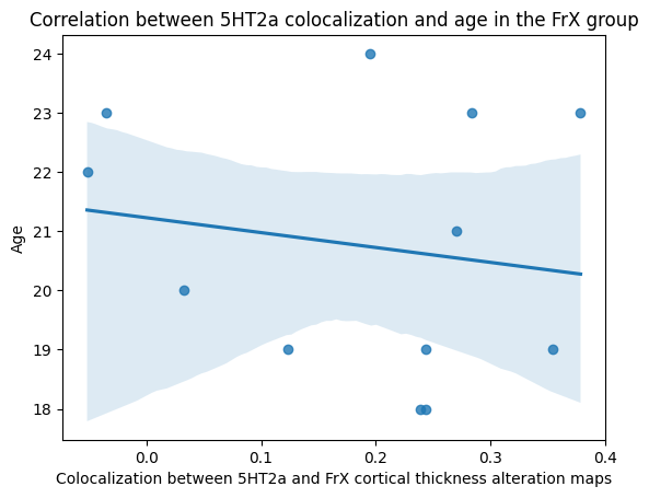
# Example:
regplot(
    x=colocs_5HT2a,
    y=df_participants.age[df_participants.diagnosis == "FrX"],
)
plt.ylabel("Age")
plt.xlabel("Colocalization between 5HT2a and FrX cortical thickness alteration maps")
_ = plt.title("Correlation between 5HT2a colocalization and age in the FrX group")

Add-on: Gene-set enrichment

We found that cortical thickness alterations in fragile X syndrome are spatially associated with serotonergic and GABAergic receptor distributions, which are two of the major cortical transmitter systems. Furthermore, we observed associations to transmitter system-overarching components (synaptic density, transcriptomic activity).

We could now ask if we can further specify this, possibly system-unspecific, association. Instead of the PET data, we can also use transcriptomic data as a reference. These have the major disadvantage of being very indirect and postmortem measurements, however, we here gain the possibility of checking spatial associations to transcriptomic distributions of many individual genes or sets of genes.

NiSpace currently includes two transcriptomic datasets: They both were build from the Allen Human Brain Atlas (AHBA), the first (“mrna”) using the abagen toolbox, the second (“magicc”) using the data provided by Wagstyl et al., 2024 (https://doi.org/10.7554/eLife.86933.1). We will go with the magicc dataset for now.

Neuroimaging gene-set enrichment analysis checks if a set of genes (e.g. 20 genes associated with vesicle trafficking) correlate more strongly with an outcome of interest (e.g., our FrX effect size map) than expected by chance. Our gene sets will be defined by the SynGO dataset, which consists of gene sets sorted by their implications in specific synaptic functions.

Get effect size map from another analysis

We will perform our analysis on a parcel-wise hedge’s g effect size map from the very first analysis.

# get FrX vs HC effect size map from another analysis (no colocalization performed yet)
effect_sizes = nsp_object_es.get_y(Y_transform="hedges(a,b)")

# show effect size map (left hemisphere: first 74 parcels)
view_surf(effect_sizes.iloc[:, :74], parcellation="Destrieux", template="fsaverage", hemi="L")

INFO | 15/06/25 16:40:48 | nispace: Loading cortex parcellation 'Destrieux' in 'fsaverage' space.

Run the analysis

We will run the X-set enrichment analysis (XSEA) workflow function. Called like below, it will automatically fetch the “magicc” reference data (as opposed to above, where we called the PET data independently before). The SynGO dataset is defined via the “x_collection” parameter and the special “set_size_range” parameter is used to only include gene sets with a size between 10 and inf genes (to exclude sets with only 1-9 genes).

from nispace.workflows import simple_xsea

# perform gene-set enrichment analysis
colocs_xsea, pvalues_xsea, qvalues_xsea, nsp_xsea = simple_xsea(
    y=effect_sizes,
    x="magicc",
    x_collection="SynGO",
    fetch_x_kwargs={"set_size_range": (10, None)},
    parcellation="Destrieux",
    colocalization_method="pls",
    permute_sets=True,
    n_perm=10000,
    n_proc=-1,
    verbose=True,
    plot=False
)

INFO | 15/06/25 16:40:48 | nispace: Trying to fetch background X dataset.
INFO | 15/06/25 16:40:48 | nispace: Loading magicc maps.
INFO | 15/06/25 16:40:48 | nispace: Loading data parcellated with 'Destrieux'
INFO | 15/06/25 16:40:48 | nispace: Using integrated parcellation Destrieux.
INFO | 15/06/25 16:40:48 | nispace: Loading integrated magicc dataset as X data.
INFO | 15/06/25 16:40:48 | nispace: Loading magicc maps.
INFO | 15/06/25 16:40:48 | nispace: Applying collection filter from: /Users/llotter/nispace-data/reference/magicc/collection-SynGO.collect.
INFO | 15/06/25 16:40:56 | nispace: Filtering to collection sets with between 10 and inf maps.
INFO | 15/06/25 16:41:00 | nispace: Loading data parcellated with 'Destrieux'
The NiSpace "magicc" dataset is based on Allen Human Brain Atlas (AHBA) gene expression data published in Hawrylycz et al.,
2012 (https://doi.org/10.1038/nature11405). The dataset consists of mRNA expression data from postmortem brain tissue of
six donors, mapped onto continuous fsLR space as described in Wagstyl et al., 2024 (https://doi.org/10.7554/eLife.86933.1),
and parcellated with integrated parcellation. Only genes that showed a high reproducibility (>= 0.5, see paper) were retained.
In addition to the two publications listed above, please cite publications associated with gene set collections as appropriate.
To ensure reproducibility, note the NiSpace commit/version: 2cb3a7f5c1cea6417fe7613465a1c503f77c87c6

- SynGO  Source: Koopmans2019  https://doi.org/10.1016/j.neuron.2019.05.002

INFO | 15/06/25 16:41:00 | nispace: *** NiSpace.fit() - Data extraction and preparation. ***
INFO | 15/06/25 16:41:00 | nispace: Loading cortex parcellation 'Destrieux' in 'MNI152NLin2009cAsym' space.
INFO | 15/06/25 16:41:00 | nispace: Loaded integrated parcellation with pre-calculated distance matrix.
INFO | 15/06/25 16:41:00 | nispace: Checking input data for 'x' (should be, e.g., PET data):
INFO | 15/06/25 16:41:00 | nispace: Input type: DataFrame, assuming parcellated data with shape (n_files/subjects/etc, n_parcels).
INFO | 15/06/25 16:41:00 | nispace: Got 'x' data for 9030 x 148 parcels.
INFO | 15/06/25 16:41:00 | nispace: Checking input data for 'y' (should be, e.g., subject data):
INFO | 15/06/25 16:41:00 | nispace: Input type: DataFrame, assuming parcellated data with shape (n_files/subjects/etc, n_parcels).
INFO | 15/06/25 16:41:00 | nispace: Got 'y' data for 1 x 148 parcels.
INFO | 15/06/25 16:41:00 | nispace: Z-standardizing 'X' data.
INFO | 15/06/25 16:41:00 | nispace: *** NiSpace.colocalize() - Estimating X & Y colocalizations. ***
INFO | 15/06/25 16:41:00 | nispace: Running 'pls' colocalization.
INFO | 15/06/25 16:41:00 | nispace: Will perform X-set enrichment analysis (XSEA).
INFO | 15/06/25 16:41:00 | nispace: Using 119 sets with between 10 and 1178 samples. Aggregating within-set colocalizations with: mean.

Colocalizing (pls, -1 proc): 100%|██████████| 1/1 [00:00<00:00, 837.52it/s]

INFO | 15/06/25 16:41:00 | nispace: *** NiSpace.permute() - Estimate exact non-parametric p values. ***
INFO | 15/06/25 16:41:00 | nispace: Permutation of: X sets.
INFO | 15/06/25 16:41:00 | nispace: Loading observed colocalizations (method = 'pls').
INFO | 15/06/25 16:41:00 | nispace: Generating permuted X sets.
INFO | 15/06/25 16:41:00 | nispace: Will use 11146 provided background maps.
INFO | 15/06/25 16:41:00 | nispace: Z-standardizing X background maps.

Permuting X set indices: 100%|██████████| 10000/10000 [00:06<00:00, 1502.77it/s]
Null colocalizations (pls, -1 proc): 100%|██████████| 10000/10000 [03:10<00:00, 52.56it/s]

INFO | 15/06/25 16:44:17 | nispace: Calculating exact p-values (tails = {'r2': 'upper', 'beta': 'two'}).
INFO | 15/06/25 16:44:18 | nispace: *** NiSpace.correct_p() - Correct p values for multiple comparisons. ***
INFO | 15/06/25 16:44:18 | nispace: Returning colocalizations:
| METHOD | XSEA | X_REDUCTION | Y_TRANSFORM |
| pls    | True | False       | False       | 
INFO | 15/06/25 16:44:18 | nispace: Returning p values:
| METHOD | PERMUTE_WHAT | XSEA | MC_METHOD | NORM  | X_REDUCTION | Y_TRANSFORM |
| pls    | sets         | True | None      | False | False       | False       | 
INFO | 15/06/25 16:44:18 | nispace: Returning p values:
| METHOD | PERMUTE_WHAT | XSEA | MC_METHOD | NORM  | X_REDUCTION | Y_TRANSFORM |
| pls    | sets         | True | fdrbh     | False | False       | False       | 

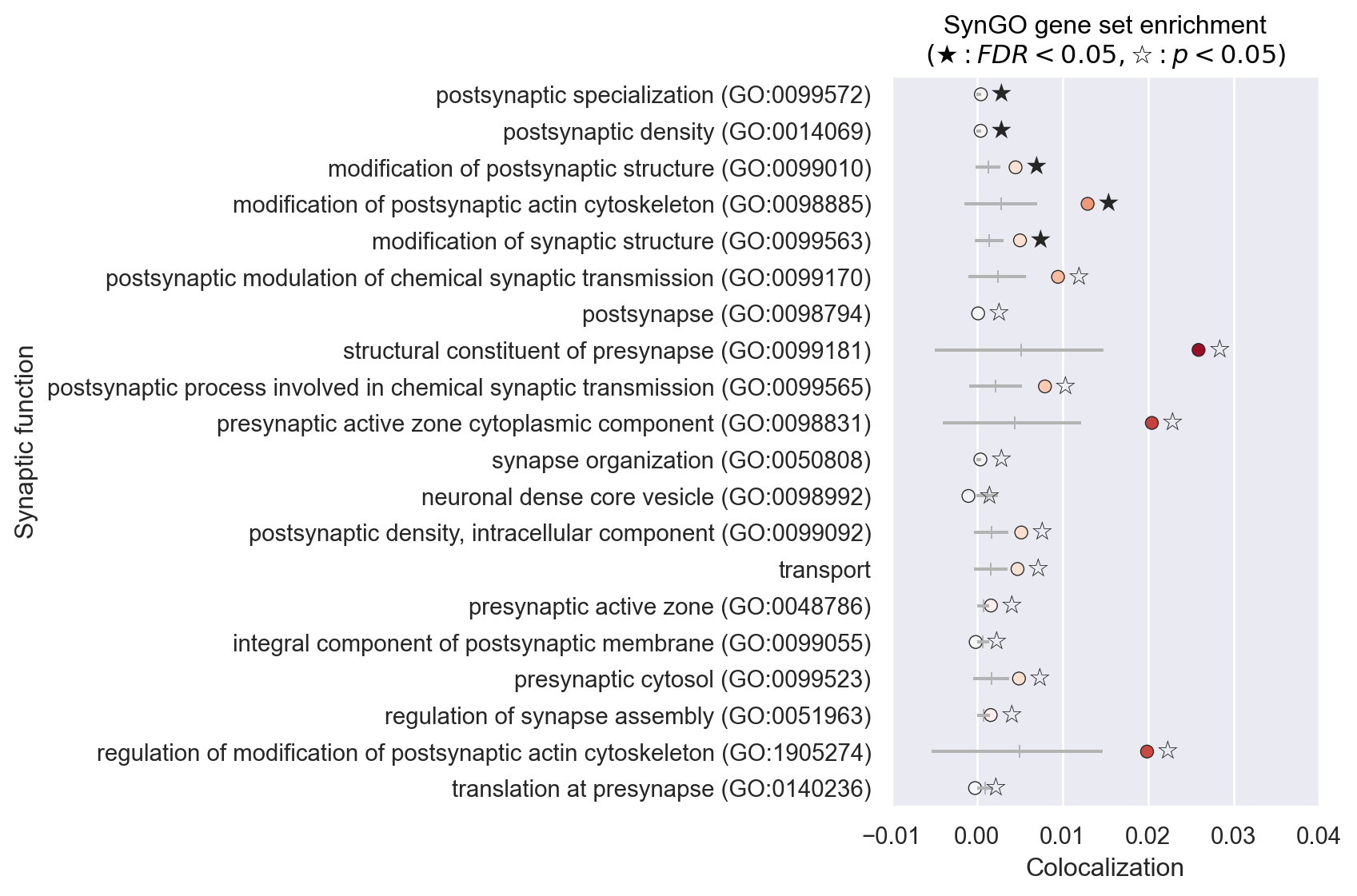
We take a look at the FDR-corrected results: We find some significant results and can generally confirm our result on the spatial association to synaptic density at the postsynapse and possibly synaptic structure.

We might therefore preliminarily conclude that we deal with a rather fundamental structural synaptic dysfunction in fragile X syndrome, rather than with a dysfunction of a specific transmitter system.

# the chosen method, PLS, will return results as dicts with two data frames: beta and r2
# we look at beta

qvalues_xsea["beta"].loc["hedges"].sort_values().head(10)

postsynaptic specialization (GO:0099572)                                        0.007933
postsynaptic density (GO:0014069)                                               0.007933
modification of postsynaptic structure (GO:0099010)                             0.007933
modification of postsynaptic actin cytoskeleton (GO:0098885)                    0.035700
modification of synaptic structure (GO:0099563)                                 0.038080
postsynaptic modulation of chemical synaptic transmission (GO:0099170)          0.067433
postsynapse (GO:0098794)                                                        0.068000
structural constituent of presynapse (GO:0099181)                               0.068425
postsynaptic process involved in chemical synaptic transmission (GO:0099565)    0.077891
synapse organization (GO:0050808)                                               0.077891
Name: hedges, dtype: float32

Plot the results

We now plot all results that are uncorrected significant for an overview. We could do that, as we did automatically in the workflow function above, by calling .plot() on the nispace object. However, as this will produce a very big plot with many categories, we will do it manually here, and only for FDR-corrected results. The function to produce adequate plots for this kind of data is currently not implemented in NiSpace.

import seaborn.objects as so

# create a dataframe with the null distribution
plot_data_null = (
    pd.concat(nsp_xsea.get_colocalizations(get_nulls=True, stats="beta", nulls_permute_what="sets")[1])
    .droplevel(1)
)
display(plot_data_null.head(3))

# create a dataframe with the results
plot_data = pd.DataFrame(
    {
        "set": colocs_xsea["beta"].columns,
        "coloc": colocs_xsea["beta"].loc["hedges"],
        "p": pvalues_xsea["beta"].loc["hedges"],
        "q": qvalues_xsea["beta"].loc["hedges"],
        "null_median": plot_data_null.median(axis=1),
        "null_pi10": plot_data_null.quantile(0.1, axis=1),
        "null_pi90": plot_data_null.quantile(0.9, axis=1),
    }
)
plot_data = plot_data.query("p < 0.05").sort_values("q")
display(plot_data.head(3))

# plot
(
    so.Plot(
        plot_data, # subset data to only include uncorrected significant results
        x="coloc",
        y="set",
        color="coloc",
        text=["$★$" if q < 0.05 else "$☆$" if p < 0.05 else "" for q, p in zip(plot_data.q, plot_data.p)],
    )
    .add(so.Range(color="0.7"), xmin="null_pi10", xmax="null_pi90", legend=False)
    .add(so.Dot(marker="|", color="0.7"), x="null_median", legend=False)
    .add(so.Dot(edgecolor="k"), legend=False)
    .add(so.Text(color="k", valign="center", halign="left", offset=4))
    .scale(color=so.Continuous("RdBu_r", norm=(-0.03, 0.03)))
    .limit(x=(-0.01, 0.04))
    .label(x="Colocalization", y="Synaptic function", title="SynGO gene set enrichment\n$(★: FDR < 0.05, ☆: p < 0.05)$")
    .layout(size=(9, 6))
    .plot()
)

INFO | 15/06/25 16:44:22 | nispace: Returning colocalizations:
| METHOD | XSEA | X_REDUCTION | Y_TRANSFORM |
| pls    | True | False       | False       | 

	0	1	2	3	4	5	6	7	8	9	...	9990	9991	9992	9993	9994	9995	9996	9997	9998	9999
synapse (GO:0045202)	0.000069	0.000057	0.000056	0.000075	0.000061	0.000056	0.000065	0.000052	0.000051	0.000049	...	0.000057	0.000054	0.000056	0.000053	0.000062	0.000053	0.000051	0.000039	0.000048	0.000066
synaptic membrane (GO:0097060)	0.001373	0.003137	0.005443	0.002388	0.004345	0.003215	-0.002482	0.003836	0.001134	-0.003315	...	0.004754	0.000042	0.002674	0.002272	0.003590	0.007391	0.004566	0.003540	0.004273	0.000693
integral component of synaptic membrane (GO:0099699)	0.001572	0.003478	0.002361	0.008681	-0.000088	0.009003	0.005905	0.017981	0.004984	0.010426	...	0.011871	0.005010	0.001870	0.013045	0.003327	0.009240	-0.001340	0.014197	0.004886	0.006027

3 rows × 10000 columns

	set	coloc	p	q	null_median	null_pi10	null_pi90
postsynaptic specialization (GO:0099572)	postsynaptic specialization (GO:0099572)	0.000446	0.0002	0.007933	0.000216	0.000135	0.000299
postsynaptic density (GO:0014069)	postsynaptic density (GO:0014069)	0.000422	0.0001	0.007933	0.000186	0.000120	0.000250
modification of postsynaptic structure (GO:0099010)	modification of postsynaptic structure (GO:009...	0.004506	0.0002	0.007933	0.001295	0.000012	0.002526