Getting started: the NiSpace object

This notebook introduces the core NiSpace API through a complete, step-by-step colocalization analysis. If you haven’t already, have a look at the Spatial Colocalization notebook for the conceptual background.

We’ll use a NeuroQuery meta-analytic map for “pain” as our input and test whether it colocalizes with a set of PET-derived neurotransmitter receptor maps. This is a clean, self-contained example with a nice biological story.

[1]:

# make progress bars render as text in the docs
import tqdm.notebook
tqdm.notebook.tqdm = tqdm.tqdm

The input map: a NeuroQuery pain map

We need a brain map to start with. I downloaded a meta-analytic map from NeuroQuery — a tool that generates brain activation maps from text queries against the neuroimaging literature. The map for “pain” is a z-score image reflecting how consistently the pain literature reports activation across brain regions.

Technically this is not a T-map from a single study, but it serves our purpose perfectly: it’s a plausible spatial pattern of pain-related brain activity, and it lives in MNI space like all our reference data.

[2]:

from nispace.io import load_img
from nispace.plotting import brainplot

# load the pain map
pain_map = load_img("neuroquery/pain.nii.gz")

# plot it
brainplot(pain_map, title="Pain (NeuroQuery)")

WARNING | 01/06/26 15:02:51 | nispace.plotting: Brain plotting in NiSpace is experimental. If things look off, feel free to raise a GitHub issue!

[2]:

(<Figure size 720x180 with 6 Axes>, [<Axes: >])

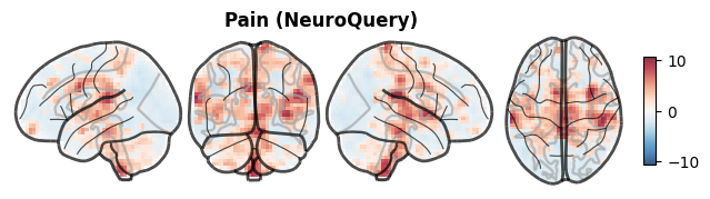
../_images/nb_introduction_intro02_nispace_intro_3_2.png

The map shows the expected pattern: activation in regions associated with pain processing, including the insula, anterior cingulate cortex, and somatosensory cortex.

Reference data: PET receptor maps

For our reference maps, we’ll use NiSpace’s curated PET receptor dataset. This collection contains group-average receptor density maps for a wide range of neurotransmitter receptors and transporters, derived from PET studies in healthy subjects.

We fetch the data already parcellated into our target parcellation. This is much faster than loading the volumetric images and parcellating them on the fly — NiSpace ships pre-parcellated versions of all reference datasets.

[3]:

from nispace.datasets import fetch_reference

# fetch the PET maps, pre-parcellated into Schaefer200
# collection="UniqueTracers" picks one representative tracer per receptor target
pet_maps = fetch_reference(
    "pet",
    parcellation="Schaefer200",
    collection="UniqueTracers",
    print_references=False  # suppress the long reference list for now
)

print(f"PET DataFrame: {pet_maps.shape[0]} maps x {pet_maps.shape[1]} parcels")
pet_maps.head(3)

INFO | 01/06/26 15:02:52 | nispace.datasets: Loading pet maps.
INFO | 01/06/26 15:02:52 | nispace.datasets: Loading integrated collection 'UniqueTracers' for dataset 'pet'.
INFO | 01/06/26 15:02:52 | nispace.datasets: Filtering maps by collection.
INFO | 01/06/26 15:02:52 | nispace.datasets: Loading data parcellated with 'Schaefer200Parcels7Networks'
PET DataFrame: 29 maps x 200 parcels

[3]:

		hemi-L_div-Vis_lab-1	hemi-L_div-Vis_lab-2	hemi-L_div-Vis_lab-3	hemi-L_div-Vis_lab-4	hemi-L_div-Vis_lab-5	hemi-L_div-Vis_lab-6	hemi-L_div-Vis_lab-7	hemi-L_div-Vis_lab-8	hemi-L_div-Vis_lab-9	hemi-L_div-Vis_lab-10	...	hemi-R_div-Default_lab-PFCm+1	hemi-R_div-Default_lab-PFCm+2	hemi-R_div-Default_lab-PFCm+3	hemi-R_div-Default_lab-PFCm+4	hemi-R_div-Default_lab-PFCm+5	hemi-R_div-Default_lab-PFCm+6	hemi-R_div-Default_lab-PFCm+7	hemi-R_div-Default_lab-PCC+1	hemi-R_div-Default_lab-PCC+2	hemi-R_div-Default_lab-PCC+3
set	map
General	target-CMRglu_tracer-fdg_n-20_dx-hc_pub-castrillon2023	0.677147	0.666611	0.633823	0.712379	0.604150	0.590683	0.707724	0.684077	0.621863	0.791744	...	0.694831	0.702473	0.573170	0.615872	0.563187	0.712010	0.677833	0.759205	0.874840	0.805161
	target-rCPS_tracer-leucine_n-42_dx-hc_pub-smith2023	0.602272	0.624987	0.600528	0.611747	0.642787	0.490786	0.707251	0.654593	0.710693	0.726193	...	0.518188	0.542567	0.537646	0.528138	0.485648	0.587230	0.521042	0.562560	0.627642	0.603664
	target-SV2A_tracer-ucbj_n-76_dx-hc_pub-finnema2016	0.651551	0.606582	0.616104	0.570561	0.536395	0.509607	0.563901	0.675601	0.618253	0.649548	...	0.702999	0.730201	0.606722	0.638996	0.551071	0.654981	0.587189	0.631831	0.721953	0.708995

3 rows × 200 columns

The DataFrame has a two-level index: the first level is the neurotransmitter system (“set”), the second is the full tracer identifier. These sets are used later for X-Set Enrichment Analysis (XSEA notebook) — for now we just treat the whole thing as a collection of maps.

Initializing the NiSpace object

NiSpace follows an object-oriented design. We first create a NiSpace instance, passing all the data and configuration options. Processing happens later when we call the analysis methods.

The two central arguments are:

x: the reference maps (here: PET receptor maps)
y: the input map(s) we want to analyze (here: the pain map)

We also specify the parcellation, which tells NiSpace how to parcellate y (since it’s a volumetric NIfTI image) and how to align it with x (which is already a parcellated DataFrame).

[4]:

from nispace.api import NiSpace

nsp = NiSpace(
    x=pet_maps,        # reference maps
    y=pain_map,        # input map — will be parcellated automatically
    y_labels="Pain",   # a name for our input map
    parcellation="Schaefer200",
    n_proc=4,          # use 4 parallel processes where possible
    seed=42            # for reproducibility
)

print(nsp)

<nispace.api.NiSpace object at 0x168d168e0>

Fitting: parcellation and data ingestion

Calling fit() is where actual data processing begins. For the pain map (a NIfTI image), this means parcellating it into the 200 Schaefer regions. For the PET maps (already a DataFrame), it validates and stores the data.

[5]:

nsp.fit()

# inspect the parcellated pain map
print("Parcellated pain map:")
nsp.get_y()

INFO | 01/06/26 15:02:52 | nispace.api: *** NiSpace.fit() - Data extraction and preparation. ***
INFO | 01/06/26 15:02:52 | nispace.core.parcellation: Building multi-space Parcellation for 'Schaefer200Parcels7Networks' from library.
INFO | 01/06/26 15:02:52 | nispace.core.parcellation: Available spaces: MNI152NLin2009cAsym, MNI152NLin6Asym, fsaverage, fsLR
INFO | 01/06/26 15:02:52 | nispace.core.parcellation: Parcellation 'Schaefer200Parcels7Networks': validation passed.
INFO | 01/06/26 15:02:52 | nispace.core.parcellation: Lazy-loading parcellation image for space 'MNI152NLin2009cAsym'.
INFO | 01/06/26 15:02:52 | nispace.core.parcellation: Parcellation 'Schaefer200Parcels7Networks': active space set to 'MNI152NLin2009cAsym'.
INFO | 01/06/26 15:02:52 | nispace.api: Checking input data for 'x' (should be, e.g., PET data):
INFO | 01/06/26 15:02:52 | nispace.io: Input type: DataFrame, assuming parcellated data with shape (n_files/subjects/etc, n_parcels).
WARNING | 01/06/26 15:02:52 | nispace.io: Parcellated data contains nan values!
INFO | 01/06/26 15:02:52 | nispace.api: Got 'x' data for 29 x 200 parcels.
INFO | 01/06/26 15:02:52 | nispace.api: Checking input data for 'y' (should be, e.g., subject data):
INFO | 01/06/26 15:02:52 | nispace.io: Input type: list, assuming imaging data.
INFO | 01/06/26 15:02:52 | nispace.io: Background (bg) handling: ignoring bg: True (bg value: ['auto', 0.0]); dropping bg parcels: False
INFO | 01/06/26 15:02:52 | nispace.io: Parcellating imaging data.

Parcellating (4 proc): 100%|████████████████████████████████████████████████████████████████████████████████████████████████████████████████████████████| 1/1 [00:00<00:00, 100.79it/s]

INFO | 01/06/26 15:02:56 | nispace.api: Got 'y' data for 1 x 200 parcels.
INFO | 01/06/26 15:02:56 | nispace.api: Z-standardizing 'X' data.
Parcellated pain map:
INFO | 01/06/26 15:02:56 | nispace.api: Returning Y dataframe:
| Y_TRANSFORM |
| False       |

[5]:

	hemi-L_div-Vis_lab-1	hemi-L_div-Vis_lab-2	hemi-L_div-Vis_lab-3	hemi-L_div-Vis_lab-4	hemi-L_div-Vis_lab-5	hemi-L_div-Vis_lab-6	hemi-L_div-Vis_lab-7	hemi-L_div-Vis_lab-8	hemi-L_div-Vis_lab-9	hemi-L_div-Vis_lab-10	...	hemi-R_div-Default_lab-PFCm+1	hemi-R_div-Default_lab-PFCm+2	hemi-R_div-Default_lab-PFCm+3	hemi-R_div-Default_lab-PFCm+4	hemi-R_div-Default_lab-PFCm+5	hemi-R_div-Default_lab-PFCm+6	hemi-R_div-Default_lab-PFCm+7	hemi-R_div-Default_lab-PCC+1	hemi-R_div-Default_lab-PCC+2	hemi-R_div-Default_lab-PCC+3
Pain	-0.436623	-1.075635	-0.893094	-0.887707	-1.139506	-1.259002	-1.339256	-1.083586	-1.389717	-0.828569	...	-0.463824	-0.154211	0.643321	-0.584073	-0.205924	0.174392	0.172215	-0.319737	-0.818837	-0.344202

1 rows × 200 columns

The parcellated data is stored internally. get_y() returns the input maps, get_x() returns the reference maps — both as DataFrames with maps in rows and parcels in columns.

Colocalization

Now for the core step: computing correlations between the pain map and each PET receptor map. We use Spearman rank correlation, which is robust to outliers and doesn’t assume normally distributed data.

[6]:

nsp.colocalize("spearman")

# get the results
colocs = nsp.get_colocalizations()
print(f"Results: {colocs.shape[0]} input maps x {colocs.shape[1]} reference maps")

# show sorted by colocalization value
colocs.T.sort_values(by="Pain", ascending=False)

INFO | 01/06/26 15:02:56 | nispace.api: *** NiSpace.colocalize() - Estimating X & Y colocalizations. ***
INFO | 01/06/26 15:02:56 | nispace.api: Running 'spearman' colocalization.
INFO | 01/06/26 15:02:56 | nispace.api: Pre-ranking X and Y data.

Colocalizing (spearman, 4 proc): 100%|█████████████████████████████████████████████████████████████████████████████████████████████████████████████████| 1/1 [00:00<00:00, 1451.32it/s]

INFO | 01/06/26 15:02:59 | nispace.api: Returning colocalizations:
| METHOD   | XSEA  | X_REDUCTION | Y_TRANSFORM |
| spearman | False | False       | False       | 
Results: 1 input maps x 29 reference maps

[6]:

		Pain
set	map
Noradrenaline/Acetylcholine	target-VAChT_tracer-feobv_n-18_dx-hc_pub-aghourian2017	0.435971
Opioids/Endocannabinoids	target-KOR_tracer-ly2795050_n-28_dx-hc_pub-vijay2018	0.339014
Noradrenaline/Acetylcholine	target-NET_tracer-mrb_n-10_dx-hc_pub-hesse2017	0.309315
Histamine	target-H3_tracer-gsk189254_n-8_dx-hc_pub-gallezot2017	0.304823
Glutamate	target-mGluR5_tracer-abp688_n-73_dx-hc_pub-smart2019	0.219451
Serotonin	target-5HTT_tracer-dasb_n-18_dx-hc_pub-savli2012	0.176491
Opioids/Endocannabinoids	target-MOR_tracer-carfentanil_n-204_dx-hc_pub-kantonen2020	0.151909
Dopamine	target-DAT_tracer-fpcit_n-174_dx-hc_pub-dukart2018	0.129229
GABA	target-GABAa5_tracer-ro154513_n-10_dx-hc_pub-lukow2022	0.111743
Opioids/Endocannabinoids	target-CB1_tracer-omar_n-77_dx-hc_pub-normandin2015	0.102278
Dopamine	target-D1_tracer-sch23390_n-13_dx-hc_pub-kaller2017	0.078620
Serotonin	target-5HT1a_tracer-way100635_n-35_dx-hc_pub-savli2012	0.073410
General	target-VMAT2_tracer-dtbz_n-76_dx-hc_pub-larsen2020	0.062397
Dopamine	target-D23_tracer-flb457_n-55_dx-hc_pub-sandiego2015	0.059017
Noradrenaline/Acetylcholine	target-A4B2_tracer-flubatine_n-30_dx-hc_pub-hillmer2016	0.036321
Dopamine	target-FDOPA_tracer-fluorodopa_n-12_dx-hc_pub-garciagomez2018	-0.000303
General	target-SV2A_tracer-ucbj_n-76_dx-hc_pub-finnema2016	-0.068091
Serotonin	target-5HT4_tracer-sb207145_n-59_dx-hc_pub-beliveau2017	-0.089016
Noradrenaline/Acetylcholine	target-M1_tracer-lsn3172176_n-24_dx-hc_pub-naganawa2020	-0.122528
Glutamate	target-NMDA_tracer-ge179_n-29_dx-hc_pub-galovic2021	-0.127164
Immunity	target-TSPO_tracer-pbr28_n-6_dx-hc_pub-lois2018	-0.134217
Immunity	target-COX1_tracer-ps13_n-11_dx-hc_pub-kim2020	-0.142131
General	target-CMRglu_tracer-fdg_n-20_dx-hc_pub-castrillon2023	-0.162803
General	target-HDAC_tracer-martinostat_n-8_dx-hc_pub-wey2016	-0.170727
GABA	target-GABAa_tracer-flumazenil_n-6_dx-hc_pub-dukart2018	-0.202272
Serotonin	target-5HT6_tracer-gsk215083_n-30_dx-hc_pub-radhakrishnan2018	-0.264142
General	target-rCPS_tracer-leucine_n-42_dx-hc_pub-smith2023	-0.274733
Serotonin	target-5HT1b_tracer-p943_n-23_dx-hc_pub-savli2012	-0.316360
Serotonin	target-5HT2a_tracer-altanserin_n-19_dx-hc_pub-savli2012	-0.328132

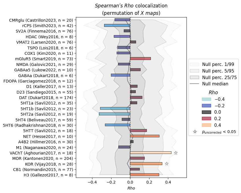
The result is a DataFrame with one row per input map (here: “Pain”) and one column per reference map. The values are Spearman ρ.

We can see which receptors show the strongest positive and negative colocalizations. But these bare correlation values don’t come with reliable p-values yet — we haven’t accounted for spatial autocorrelation. That’s where permutation testing comes in.

Permutation testing

We call permute() with "maps" to generate spatially-constrained null versions of the PET maps and recompute correlations 10,000 times. This gives us an empirical null distribution for each receptor.

We pass p_tails="upper" because our hypothesis is directional: we expect positive colocalizations with receptors involved in pain processing (opioids, noradrenergic/cholinergic pathways).

Null model details are covered in the Null Models notebook. For now, just note that by default NiSpace uses spin-based surrogate maps if possible (Alexander-Bloch method), which preserve the spatial autocorrelation of the original data.

[7]:

nsp.permute(
    "maps",
    n_perm=1000, # increase to >=10000 for final analyses
    p_tails="upper",  # one-tailed: test for positive colocalization, default is "two"
)

# multiple comparison correction across the 29 receptor maps
nsp.correct_p() # mc_method argument to specify method, default is "meff" (effective number of tests)

p_values = nsp.get_p_values()

# show p-values sorted ascending
p_values.T.sort_values(by="Pain")

INFO | 01/06/26 15:02:59 | nispace.api: *** NiSpace.permute() - Estimate exact non-parametric p values. ***
INFO | 01/06/26 15:02:59 | nispace.api: Permutation of: X maps.
INFO | 01/06/26 15:02:59 | nispace.api: Using default null method 'alexander_bloch' (parcellation null space: 'fsLR').
INFO | 01/06/26 15:02:59 | nispace.core.parcellation: Lazy-loading parcellation image for space 'fsLR'.
INFO | 01/06/26 15:02:59 | nispace.api: Loading observed colocalizations (method = 'spearman').
INFO | 01/06/26 15:02:59 | nispace.api: Returning colocalizations:
| METHOD   | XSEA  | X_REDUCTION | Y_TRANSFORM |
| spearman | False | False       | False       | 
INFO | 01/06/26 15:02:59 | nispace.api: Generating permuted X maps.
INFO | 01/06/26 15:02:59 | nispace.core.permute: No null maps found.
INFO | 01/06/26 15:02:59 | nispace.core.permute: Generating null maps (n = 1000, null_method = 'alexander_bloch').
INFO | 01/06/26 15:02:59 | nispace.core.parcellation: Lazy-loading parcellation image for space 'fsaverage'.
INFO | 01/06/26 15:02:59 | nispace.nulls: Null map generation: Assuming n = 29 data vector(s) for n = 200 parcels.
INFO | 01/06/26 15:02:59 | nispace.nulls: Using provided precomputed spin matrix.

Spin null maps: 100%|█████████████████████████████████████████████████████████████████████████████████████████████████████████████████████████████████| 29/29 [00:00<00:00, 234.44it/s]

INFO | 01/06/26 15:02:59 | nispace.nulls: Null data generation finished.
INFO | 01/06/26 15:02:59 | nispace.core.permute: Z-standardizing null maps.
INFO | 01/06/26 15:02:59 | nispace.api: Pre-ranking X and Y (null) data.


Processing null arrays (4 proc): 100%|████████████████████████████████████████████████████████████████████████████████████████████████████████████| 1000/1000 [00:01<00:00, 888.56it/s]
Null colocalizations (spearman, 4 proc): 100%|███████████████████████████████████████████████████████████████████████████████████████████████████| 1000/1000 [00:00<00:00, 7792.89it/s]

INFO | 01/06/26 15:03:03 | nispace.core.permute: Calculating exact p-values (tails = {'rho': 'upper'}).
INFO | 01/06/26 15:03:03 | nispace.api: *** NiSpace.correct_p() - Correct p values for multiple comparisons. ***
INFO | 01/06/26 15:03:03 | nispace.api: Correction method: 'meff_galwey', alpha: 0.05, dimension: 'array'.
INFO | 01/06/26 15:03:03 | nispace.api: Returning X dataframe:
| X_REDUCTION |
| False       | 
INFO | 01/06/26 15:03:03 | nispace.api: Meff_X (galwey) = 12.28 (from 29 maps).
INFO | 01/06/26 15:03:03 | nispace.api: Returning p values:
| METHOD   | PERMUTE_WHAT | XSEA  | MC_METHOD | X_REDUCTION | Y_TRANSFORM |
| spearman | xmaps        | False | None      | False       | False       |

[7]:

		Pain
set	map
Noradrenaline/Acetylcholine	target-VAChT_tracer-feobv_n-18_dx-hc_pub-aghourian2017	0.020
Opioids/Endocannabinoids	target-KOR_tracer-ly2795050_n-28_dx-hc_pub-vijay2018	0.031
Noradrenaline/Acetylcholine	target-NET_tracer-mrb_n-10_dx-hc_pub-hesse2017	0.068
Histamine	target-H3_tracer-gsk189254_n-8_dx-hc_pub-gallezot2017	0.075
Glutamate	target-mGluR5_tracer-abp688_n-73_dx-hc_pub-smart2019	0.167
Serotonin	target-5HTT_tracer-dasb_n-18_dx-hc_pub-savli2012	0.227
Opioids/Endocannabinoids	target-MOR_tracer-carfentanil_n-204_dx-hc_pub-kantonen2020	0.254
Dopamine	target-DAT_tracer-fpcit_n-174_dx-hc_pub-dukart2018	0.272
Opioids/Endocannabinoids	target-CB1_tracer-omar_n-77_dx-hc_pub-normandin2015	0.325
GABA	target-GABAa5_tracer-ro154513_n-10_dx-hc_pub-lukow2022	0.334
Dopamine	target-D1_tracer-sch23390_n-13_dx-hc_pub-kaller2017	0.347
General	target-VMAT2_tracer-dtbz_n-76_dx-hc_pub-larsen2020	0.376
Serotonin	target-5HT1a_tracer-way100635_n-35_dx-hc_pub-savli2012	0.400
Dopamine	target-D23_tracer-flb457_n-55_dx-hc_pub-sandiego2015	0.410
Noradrenaline/Acetylcholine	target-A4B2_tracer-flubatine_n-30_dx-hc_pub-hillmer2016	0.443
Dopamine	target-FDOPA_tracer-fluorodopa_n-12_dx-hc_pub-garciagomez2018	0.448
General	target-SV2A_tracer-ucbj_n-76_dx-hc_pub-finnema2016	0.652
Serotonin	target-5HT4_tracer-sb207145_n-59_dx-hc_pub-beliveau2017	0.657
Immunity	target-TSPO_tracer-pbr28_n-6_dx-hc_pub-lois2018	0.731
General	target-CMRglu_tracer-fdg_n-20_dx-hc_pub-castrillon2023	0.745
Noradrenaline/Acetylcholine	target-M1_tracer-lsn3172176_n-24_dx-hc_pub-naganawa2020	0.756
Glutamate	target-NMDA_tracer-ge179_n-29_dx-hc_pub-galovic2021	0.761
Immunity	target-COX1_tracer-ps13_n-11_dx-hc_pub-kim2020	0.783
GABA	target-GABAa_tracer-flumazenil_n-6_dx-hc_pub-dukart2018	0.846
General	target-HDAC_tracer-martinostat_n-8_dx-hc_pub-wey2016	0.853
General	target-rCPS_tracer-leucine_n-42_dx-hc_pub-smith2023	0.873
Serotonin	target-5HT6_tracer-gsk215083_n-30_dx-hc_pub-radhakrishnan2018	0.882
	target-5HT1b_tracer-p943_n-23_dx-hc_pub-savli2012	0.884
	target-5HT2a_tracer-altanserin_n-19_dx-hc_pub-savli2012	0.952

After correcting for spatial autocorrelation (via permutation) and for multiple comparisons across the 29 receptor maps (FDR), the cholinergic transporter VAChT stands out with the lowest p-value — consistent with the pain neuroscience literature.

Notice that the effect sizes haven’t changed: permutation testing and correct_p() only affect the p-values, not the correlations.

Visualizing the results

NiSpace has an integrated plot() method that picks a reasonable visualization automatically.

[8]:

nsp.plot()

INFO | 01/06/26 15:03:03 | nispace.api: *** NiSpace.plot() - Plot colocalization results. ***
INFO | 01/06/26 15:03:03 | nispace.api: Returning p values:
| METHOD   | PERMUTE_WHAT | XSEA  | MC_METHOD | X_REDUCTION | Y_TRANSFORM |
| spearman | xmaps        | False | None      | False       | False       | 
INFO | 01/06/26 15:03:03 | nispace.api: Returning colocalizations:
| METHOD   | XSEA  | X_REDUCTION | Y_TRANSFORM |
| spearman | False | False       | False       | 
INFO | 01/06/26 15:03:03 | nispace.api: Returning p values:
| METHOD   | PERMUTE_WHAT | XSEA  | MC_METHOD | X_REDUCTION | Y_TRANSFORM |
| spearman | xmaps        | False | None      | False       | False       | 
INFO | 01/06/26 15:03:03 | nispace.api: Returning p values:
| METHOD   | PERMUTE_WHAT | XSEA  | MC_METHOD  | X_REDUCTION | Y_TRANSFORM |
| spearman | xmaps        | False | meffgalwey | False       | False       | 
INFO | 01/06/26 15:03:03 | nispace.api: Creating categorical plot for method spearman, colocalization stat rho.
INFO | 01/06/26 15:03:03 | nispace.plotting: Significance annotation: 2/29 p_uncorrected < 0.05, 0/29 p_meffgalwey < 0.05

../_images/nb_introduction_intro02_nispace_intro_15_1.png

[8]:

(<Figure size 500x730 with 1 Axes>,
 <Axes: title={'center': "$Spearman's\\ Rho$ colocalization\n(permutation of $X\\ maps$)"}, xlabel='$Rho$'>,
 <seaborn._core.plot.Plotter at 0x3193e8bb0>)

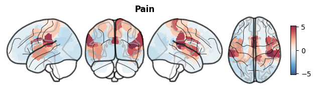
We can also visualize the input and reference maps as above, but here directly from NiSpace object:

[9]:

# the pain map
nsp.plot_brain(data="Y")

INFO | 01/06/26 15:03:03 | nispace.api: *** NiSpace.plot_brain() ***
INFO | 01/06/26 15:03:03 | nispace.api: Plotting Y data (Y_transform='False').
INFO | 01/06/26 15:03:03 | nispace.api: Returning Y dataframe:
| Y_TRANSFORM |
| False       | 
WARNING | 01/06/26 15:03:03 | nispace.plotting: Brain plotting in NiSpace is experimental. If things look off, feel free to raise a GitHub issue!
INFO | 01/06/26 15:03:03 | nispace.plotting: brainplot: threshold='auto' → 0.005351351574063301
INFO | 01/06/26 15:03:03 | nispace.plotting: brainplot: kind='glass', img_mode='None', surf_space='None', mni_space='MNI152NLin2009cAsym', surf_mesh='inflated'

../_images/nb_introduction_intro02_nispace_intro_17_1.png

[9]:

(<Figure size 720x180 with 6 Axes>, [<Axes: >])

[10]:

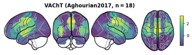
# the VAChT receptor map (strongest colocalization)
nsp.plot_brain(data="X", maps="VAChT", symmetric_cmap=False)

INFO | 01/06/26 15:03:07 | nispace.api: *** NiSpace.plot_brain() ***
INFO | 01/06/26 15:03:07 | nispace.api: Plotting X data (X_reduction='False').
INFO | 01/06/26 15:03:07 | nispace.api: Returning X dataframe:
| X_REDUCTION |
| False       | 
WARNING | 01/06/26 15:03:07 | nispace.plotting: Brain plotting in NiSpace is experimental. If things look off, feel free to raise a GitHub issue!
INFO | 01/06/26 15:03:07 | nispace.plotting: brainplot: threshold='auto' → 0.019260043278336525
INFO | 01/06/26 15:03:07 | nispace.plotting: brainplot: kind='glass', img_mode='None', surf_space='None', mni_space='MNI152NLin2009cAsym', surf_mesh='inflated'

../_images/nb_introduction_intro02_nispace_intro_18_1.png

[10]:

(<Figure size 720x180 with 6 Axes>, [<Axes: >])

Saving and loading

Analyses with 10,000 permutations take time. We can serialize the entire NiSpace object — including the null distributions — to disk with to_pickle(), and load it back with from_pickle().

We recommend the .pkl.blosc format: Blosc compression keeps file sizes manageable without the speed penalty of gzip.

[11]:

import os

# save, including the null distributions
nsp.to_pickle("nsp_pain.pkl.blosc")
print(f"With nulls:    {os.path.getsize('nsp_pain.pkl.blosc') / 1e6:.1f} MB")

# save without nulls — much smaller, but you lose the shading in plots
nsp.to_pickle("nsp_pain_no_nulls.pkl.blosc", save_nulls=False)
print(f"Without nulls: {os.path.getsize('nsp_pain_no_nulls.pkl.blosc') / 1e6:.1f} MB")

With nulls:    29.9 MB
Without nulls: 7.4 MB

[12]:

# load it back
nsp_loaded = NiSpace.from_pickle("nsp_pain.pkl.blosc")

import numpy as np
assert np.allclose(
    nsp.get_colocalizations().values,
    nsp_loaded.get_colocalizations().values
)
print("Loaded successfully — results are identical.")

INFO | 01/06/26 15:03:10 | nispace.api: Returning colocalizations:
| METHOD   | XSEA  | X_REDUCTION | Y_TRANSFORM |
| spearman | False | False       | False       | 
INFO | 01/06/26 15:03:10 | nispace.api: Returning colocalizations:
| METHOD   | XSEA  | X_REDUCTION | Y_TRANSFORM |
| spearman | False | False       | False       | 
Loaded successfully — results are identical.

Summary

The complete NiSpace workflow in six lines:

nsp = NiSpace(x=reference_maps, y=input_map, parcellation="Schaefer200")
nsp.fit()                                          # parcellate + ingest
nsp.colocalize("spearman")                         # compute correlations
nsp.permute("maps", n_perm=10000, p_tails="upper") # permutation p-values
nsp.correct_p(mc_method=...)                       # multiple comparisons correction
nsp.plot()                                         # visualize

The next notebook covers what datasets and parcellations are available, and how to bring in your own data.