Visualizing colocalization results

NiSpace has two integrated visualization methods that work directly on the fitted NiSpace object:

nsp.plot() — colocalization results (bar charts, scatter plots, …)
nsp.plot_brain() — brain surface or volume rendering of input/reference maps

This notebook walks through the customization options for both. For standalone brain plotting (independent of any NiSpace analysis), see Notebook 8.

[2]:

import tqdm.notebook
tqdm.notebook.tqdm = tqdm.tqdm

import numpy as np
import matplotlib.pyplot as plt

[3]:

from nispace.datasets import fetch_reference, fetch_example
from nispace.io import load_img
from nispace.api import NiSpace

# set up two analyses: pain map (single map) and anorexia nervosa (group comparison)
pet_maps = fetch_reference("pet", parcellation="Yan200",
                           collection="UniqueTracers", print_references=False)

# single map: pain
nsp_pain = NiSpace(x=pet_maps, y=load_img("neuroquery/pain.nii.gz"),
                   y_labels="Pain", parcellation="Yan200", seed=42, n_proc=4)
nsp_pain.fit()
nsp_pain.colocalize("spearman")
nsp_pain.permute("maps", n_perm=1000, p_tails="upper")

# group comparison: anorexia nervosa (simulated data — not for scientific use)
an_data = fetch_example("anorexianervosa", parcellation="Yan200")
groups = an_data.index.str.extract(r'(AN|HC)$')[0].values

nsp_an = NiSpace(x=pet_maps, y=an_data, parcellation="Yan200", seed=42, n_proc=4)
nsp_an.fit()
nsp_an.transform_y("hedges(a,b)", groups=groups)
nsp_an.colocalize("spearman")
nsp_an.permute("groups", groups=groups, n_perm=1000)

INFO | 20/07/26 18:21:36 | nispace.datasets: Loading pet maps.
INFO | 20/07/26 18:21:36 | nispace.datasets: Loading integrated collection 'UniqueTracers' for dataset 'pet'.
INFO | 20/07/26 18:21:36 | nispace.datasets: Filtering maps by collection.
INFO | 20/07/26 18:21:36 | nispace.datasets: Loading data parcellated with 'Yan200'
INFO | 20/07/26 18:21:36 | nispace.api: *** NiSpace.fit() - Data extraction and preparation. ***
INFO | 20/07/26 18:21:36 | nispace.core.parcellation: Building cortex Parcellation for 'Yan200' from library. DOI: 10.1016/j.neuroimage.2023.120010
INFO | 20/07/26 18:21:36 | nispace.core.parcellation: Available spaces: MNI152NLin2009cAsym, MNI152NLin6Asym, fsLR, fsaverage
INFO | 20/07/26 18:21:37 | nispace.core.parcellation: Parcellation 'Yan200': validation passed.
INFO | 20/07/26 18:21:37 | nispace.core.parcellation: Lazy-loading parcellation image for space 'MNI152NLin2009cAsym'.
INFO | 20/07/26 18:21:37 | nispace.core.parcellation: Parcellation 'Yan200': active space set to 'MNI152NLin2009cAsym'.
INFO | 20/07/26 18:21:37 | nispace.api: Checking input data for 'x' (should be, e.g., PET data):
INFO | 20/07/26 18:21:37 | nispace.io: Input type: DataFrame, assuming parcellated data with shape (n_files/subjects/etc, n_parcels).
WARNING | 20/07/26 18:21:37 | nispace.io: Parcellated data contains nan values!
INFO | 20/07/26 18:21:37 | nispace.api: Got 'x' data for 29 x 200 parcels.
INFO | 20/07/26 18:21:37 | nispace.api: Checking input data for 'y' (should be, e.g., subject data):
INFO | 20/07/26 18:21:37 | nispace.io: Input type: list, assuming imaging data.
INFO | 20/07/26 18:21:37 | nispace.io: Background (bg) handling: background_value='auto'; reporting bg-only parcels: False
INFO | 20/07/26 18:21:37 | nispace.io: Parcellating imaging data.

Parcellating (4 proc): 100%|█████████████████████████████████████████████████████████████| 1/1 [00:00<00:00, 111.90it/s]

INFO | 20/07/26 18:21:41 | nispace.api: Got 'y' data for 1 x 200 parcels.
INFO | 20/07/26 18:21:41 | nispace.api: Z-standardizing 'X' data.
INFO | 20/07/26 18:21:41 | nispace.api: *** NiSpace.colocalize() - Estimating X & Y colocalizations. ***
INFO | 20/07/26 18:21:41 | nispace.api: Running 'spearman' colocalization.
INFO | 20/07/26 18:21:41 | nispace.api: Pre-ranking X and Y data.

Colocalizing (spearman, 4 proc): 100%|██████████████████████████████████████████████████| 1/1 [00:00<00:00, 2252.58it/s]

INFO | 20/07/26 18:21:44 | nispace.api: *** NiSpace.permute() - Estimate exact non-parametric p values. ***
INFO | 20/07/26 18:21:44 | nispace.api: Permutation of: X maps.
INFO | 20/07/26 18:21:44 | nispace.api: Using default null method 'moran' (parcellation null space: 'fsLR').
INFO | 20/07/26 18:21:44 | nispace.core.parcellation: Lazy-loading parcellation image for space 'fsLR'.
INFO | 20/07/26 18:21:44 | nispace.api: Loading observed colocalizations (method = 'spearman').
INFO | 20/07/26 18:21:44 | nispace.core.permute: Generating null maps (n = 1000, null_method = 'moran').
INFO | 20/07/26 18:21:44 | nispace.nulls: Null map generation: Assuming n = 29 data vector(s) for n = 200 parcels.
INFO | 20/07/26 18:21:44 | nispace.nulls: Using provided distance matrix/matrices.

Moran null maps (4 proc): 100%|█████████████████████████████████████████████████████████| 29/29 [00:00<00:00, 56.01it/s]

INFO | 20/07/26 18:21:47 | nispace.nulls: Null data generation finished.
INFO | 20/07/26 18:21:47 | nispace.core.permute: Z-standardizing null maps.

Processing null arrays (4 proc): 100%|█████████████████████████████████████████████| 1000/1000 [00:01<00:00, 914.05it/s]
Null colocalizations (spearman, 4 proc): 100%|████████████████████████████████████| 1000/1000 [00:00<00:00, 9040.11it/s]

INFO | 20/07/26 18:21:49 | nispace.core.permute: Calculating exact p-values (tails = {'rho': 'upper'}).
INFO | 20/07/26 18:21:49 | nispace.datasets: Loading example dataset: 'anorexianervosa', parcellated with: Yan200.
INFO | 20/07/26 18:21:49 | nispace.core.parcellation: Building cortex Parcellation for 'Yan200' from library. DOI: 10.1016/j.neuroimage.2023.120010
INFO | 20/07/26 18:21:49 | nispace.core.parcellation: Available spaces: MNI152NLin2009cAsym, MNI152NLin6Asym, fsLR, fsaverage
INFO | 20/07/26 18:21:50 | nispace.core.parcellation: Parcellation 'Yan200': validation passed.
INFO | 20/07/26 18:21:50 | nispace.io: Input type: DataFrame, assuming parcellated data with shape (n_files/subjects/etc, n_parcels).
WARNING | 20/07/26 18:21:50 | nispace.io: Parcellated data contains nan values!
INFO | 20/07/26 18:21:50 | nispace.io: Input type: DataFrame, assuming parcellated data with shape (n_files/subjects/etc, n_parcels).

Colocalizing (spearman, 4 proc): 100%|██████████████████████████████████████████████████| 1/1 [00:00<00:00, 1945.41it/s]

INFO | 20/07/26 18:21:50 | nispace.core.parcellation: Lazy-loading parcellation image for space 'fsLR'.


Permuting groups (4 proc): 100%|████████████████████████████████████████████████| 1000/1000 [00:00<00:00, 728937.09it/s]
Null transformations (spearman, 4 proc): 100%|████████████████████████████████████| 1000/1000 [00:00<00:00, 3822.42it/s]
Processing null arrays (4 proc): 100%|████████████████████████████████████████████| 1000/1000 [00:00<00:00, 3799.69it/s]
Null colocalizations (spearman, 4 proc): 100%|███████████████████████████████████| 1000/1000 [00:00<00:00, 11361.81it/s]

INFO | 20/07/26 18:21:51 | nispace.core.permute: Calculating exact p-values (tails = {'rho': 'two'}).

[3]:

<nispace.api.NiSpace at 0x13fbbda90>

`nsp.plot()` — colocalization results

Default output

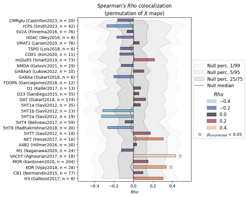
The default plot() shows a categorical bar chart of colocalization values, colored by neurotransmitter system, with the null distribution shaded in grey.

[4]:

nsp_pain.plot()

INFO | 20/07/26 18:21:52 | nispace.plotting: Significance annotation: 0/29 p_uncorrected < 0.05, 0/29 p_corrected < 0.05 (no correction applied)

../_images/nb_introduction_intro07_visualization_4_1.png

[4]:

(<Figure size 500x730 with 1 Axes>,
 <Axes: title={'center': "$Spearman's\\ Rho$ colocalization\n(permutation of $X\\ maps$)"}, xlabel='$Rho$'>,
 <seaborn._core.plot.Plotter at 0x15ffc0b80>)

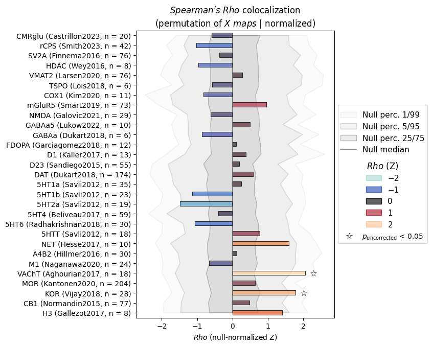
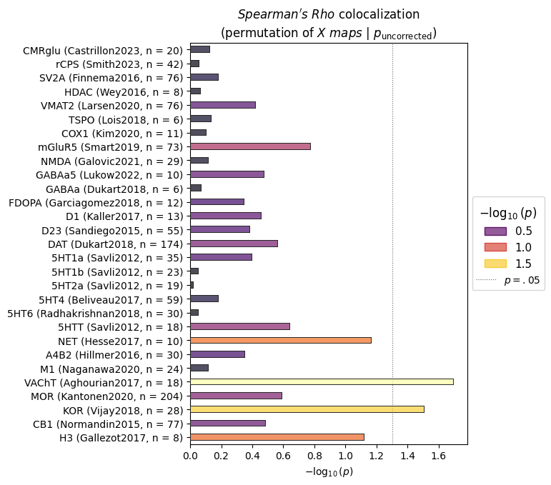
Values: raw correlations, z-scores, or -log10(p)

The values argument controls what’s shown on the x-axis:

"coloc" — raw colocalization values (Spearman ρ, partial r, …)
"z" — null-normalized z-scores (colocalization scaled by null mean and sd)
"p" — −log₁₀(p), optionally with multiple comparison correction

[5]:

# z-normalized values (makes effect sizes more comparable across maps)
nsp_pain.normalize_colocalizations() # we need to calculate the normalized scores first
nsp_pain.plot(values="z")

INFO | 20/07/26 18:21:52 | nispace.plotting: Significance annotation: 0/29 p_uncorrected < 0.05, 0/29 p_corrected < 0.05 (no correction applied)

../_images/nb_introduction_intro07_visualization_6_1.png

[5]:

(<Figure size 500x730 with 1 Axes>,
 <Axes: title={'center': "$Spearman's\\ Rho$ colocalization\n(permutation of $X\\ maps$ | normalized)"}, xlabel='$Rho$ (null-normalized Z)'>,
 <seaborn._core.plot.Plotter at 0x15fea1040>)

[6]:

# -log10(p), with FDR correction marked
nsp_pain.plot(values="p")

../_images/nb_introduction_intro07_visualization_7_0.png

[6]:

(<Figure size 500x730 with 1 Axes>,
 <Axes: title={'center': "$Spearman's\\ Rho$ colocalization\n(permutation of $X\\ maps$ | $p_{\\mathrm{uncorrected}}$)"}, xlabel='$-\\log_{10}(p)$'>,
 <seaborn._core.plot.Plotter at 0x1698bf310>)

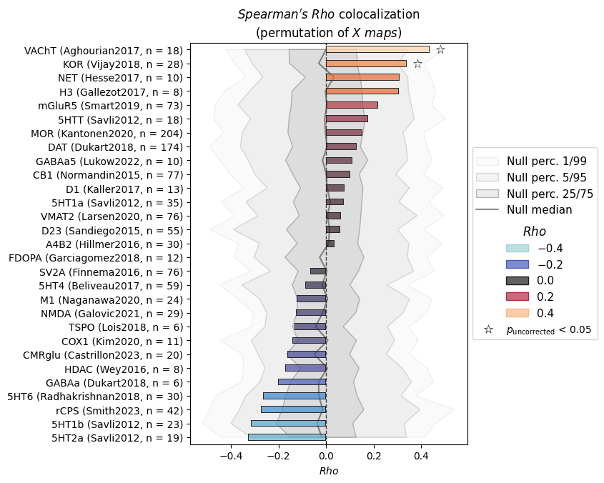
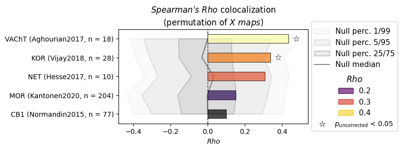
Sorting and filtering

Use sort_by to reorder the bars, and X_maps to select a subset of reference maps.

[7]:

# sort by colocalization value
nsp_pain.plot(sort_by="coloc")

INFO | 20/07/26 18:21:53 | nispace.plotting: Significance annotation: 0/29 p_uncorrected < 0.05, 0/29 p_corrected < 0.05 (no correction applied)

../_images/nb_introduction_intro07_visualization_9_1.png

[7]:

(<Figure size 500x730 with 1 Axes>,
 <Axes: title={'center': "$Spearman's\\ Rho$ colocalization\n(permutation of $X\\ maps$)"}, xlabel='$Rho$'>,
 <seaborn._core.plot.Plotter at 0x169b3aee0>)

[8]:

# show only specific systems
nsp_pain.plot(
    X_maps=["VAChT", "NET", "MOR", "KOR", "CB1"],  # match by partial name
    sort_by="coloc"
)

INFO | 20/07/26 18:21:53 | nispace.plotting: Significance annotation: 0/5 p_uncorrected < 0.05, 0/5 p_corrected < 0.05 (no correction applied)

../_images/nb_introduction_intro07_visualization_10_1.png

[8]:

(<Figure size 500x250 with 1 Axes>,
 <Axes: title={'center': "$Spearman's\\ Rho$ colocalization\n(permutation of $X\\ maps$)"}, xlabel='$Rho$'>,
 <seaborn._core.plot.Plotter at 0x169c296a0>)

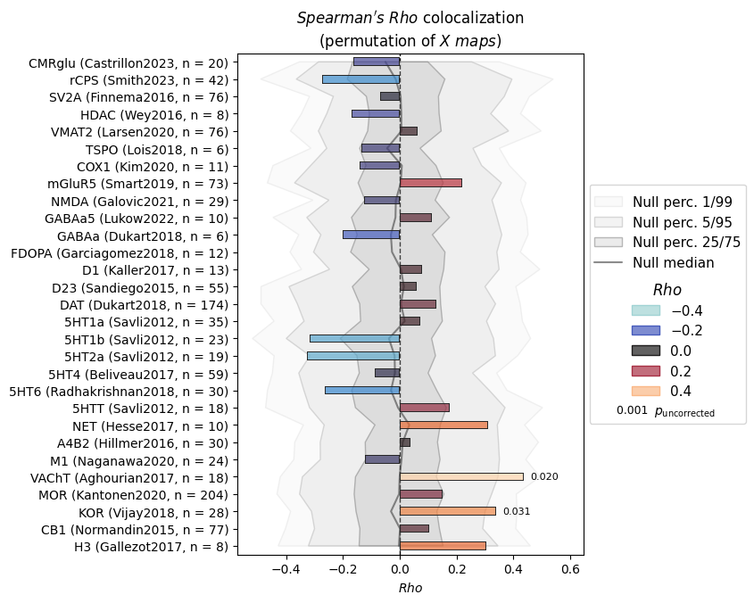
P-value annotations

annot_p controls how significance markers are shown

"stats" — show filled and empty significance stars (default; filled -> corrected; empty -> raw values)
"text" - show raw p values as text
"both" — show stars and raw p value as text
False — no markers

[9]:

nsp_pain.plot(annot_p="text")

INFO | 20/07/26 18:21:53 | nispace.plotting: Significance annotation: 0/29 p_uncorrected < 0.05, 0/29 p_corrected < 0.05 (no correction applied)

../_images/nb_introduction_intro07_visualization_12_1.png

[9]:

(<Figure size 500x730 with 1 Axes>,
 <Axes: title={'center': "$Spearman's\\ Rho$ colocalization\n(permutation of $X\\ maps$)"}, xlabel='$Rho$'>,
 <seaborn._core.plot.Plotter at 0x169dab790>)

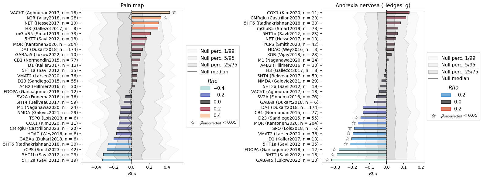
Passing to matplotlib

plot() returns (fig, ax, plot_object), so you can post-process the figure with standard matplotlib calls. You can also pass fig and ax to embed the plot in an existing figure.

[10]:

fig, axes = plt.subplots(1, 2, figsize=(16, 6))

# important: also pass the figure level, otherwise legends will behave quite unpredictably
nsp_pain.plot(ax=axes[0], fig=fig, show=False, title="Pain map", sort_by="coloc")
nsp_an.plot(ax=axes[1], fig=fig, show=False, title="Anorexia nervosa (Hedges' g)", sort_by="coloc")

plt.tight_layout()
plt.show()

INFO | 20/07/26 18:21:54 | nispace.plotting: Significance annotation: 0/29 p_uncorrected < 0.05, 0/29 p_corrected < 0.05 (no correction applied)
INFO | 20/07/26 18:21:54 | nispace.plotting: Significance annotation: 12/29 p_uncorrected < 0.05, 0/29 p_corrected < 0.05 (no correction applied)

../_images/nb_introduction_intro07_visualization_14_1.png

`nsp.plot_brain()` — brain surface rendering

Basic usage

[11]:

# plot the Y data (pain map after parcellation)
nsp_pain.plot_brain(data="Y")

WARNING | 20/07/26 18:21:54 | nispace.plotting: Brain plotting in NiSpace is experimental. If things look off, feel free to raise a GitHub issue!
INFO | 20/07/26 18:21:54 | nispace.plotting: brainplot: threshold='auto' → 0.0017398296622559428
INFO | 20/07/26 18:21:54 | nispace.plotting: brainplot: kind='glass', img_mode='None', surf_space='None', mni_space='MNI152NLin2009cAsym', surf_mesh='inflated'

../_images/nb_introduction_intro07_visualization_16_1.png

[11]:

(<Figure size 720x180 with 6 Axes>, [<Axes: >])

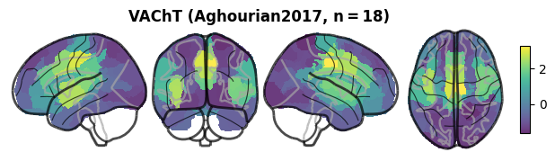
[12]:

# plot a specific reference map
nsp_pain.plot_brain(data="X", maps="VAChT", symmetric_cmap=False)

WARNING | 20/07/26 18:21:58 | nispace.plotting: Brain plotting in NiSpace is experimental. If things look off, feel free to raise a GitHub issue!
INFO | 20/07/26 18:21:58 | nispace.plotting: brainplot: threshold='auto' → 0.0001124086047639139
INFO | 20/07/26 18:21:58 | nispace.plotting: brainplot: kind='glass', img_mode='None', surf_space='None', mni_space='MNI152NLin2009cAsym', surf_mesh='inflated'

../_images/nb_introduction_intro07_visualization_17_1.png

[12]:

(<Figure size 720x180 with 6 Axes>, [<Axes: >])

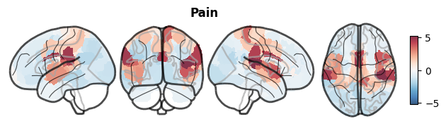
Rendering modes

The kind argument controls the rendering:

"surface" — inflated cortical surface (default for cortex-only parcellations)
"glass" — glass brain (transparent volumetric rendering)
"slice" — anatomical slices

[13]:

nsp_pain.plot_brain(data="Y", kind="glass")

WARNING | 20/07/26 18:22:01 | nispace.plotting: Brain plotting in NiSpace is experimental. If things look off, feel free to raise a GitHub issue!
INFO | 20/07/26 18:22:01 | nispace.plotting: brainplot: threshold='auto' → 0.0017398296622559428
INFO | 20/07/26 18:22:01 | nispace.plotting: brainplot: kind='glass', img_mode='None', surf_space='None', mni_space='MNI152NLin2009cAsym', surf_mesh='inflated'

../_images/nb_introduction_intro07_visualization_19_1.png

[13]:

(<Figure size 720x180 with 6 Axes>, [<Axes: >])

[14]:

nsp_pain.plot_brain(data="Y", kind="slice")

WARNING | 20/07/26 18:22:05 | nispace.plotting: Brain plotting in NiSpace is experimental. If things look off, feel free to raise a GitHub issue!
INFO | 20/07/26 18:22:05 | nispace.plotting: brainplot: threshold='auto' → 0.0017398296622559428
INFO | 20/07/26 18:22:05 | nispace.plotting: brainplot: kind='slice', img_mode='None', surf_space='None', mni_space='MNI152NLin2009cAsym', surf_mesh='inflated'

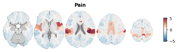
../_images/nb_introduction_intro07_visualization_20_1.png

[14]:

(<Figure size 700x180 with 7 Axes>, [<Axes: >])

Colormap and scale options

[15]:

# custom colormap, fixed scale, colorbar label
nsp_pain.plot_brain(
    data="Y",
    cmap="viridis",
    symmetric_cmap=False,
    vmin=0,
    colorbar_label="z-score"
)

WARNING | 20/07/26 18:22:09 | nispace.plotting: Brain plotting in NiSpace is experimental. If things look off, feel free to raise a GitHub issue!
INFO | 20/07/26 18:22:09 | nispace.plotting: brainplot: threshold='auto' → 0.0017398296622559428
INFO | 20/07/26 18:22:09 | nispace.plotting: brainplot: kind='glass', img_mode='None', surf_space='None', mni_space='MNI152NLin2009cAsym', surf_mesh='inflated'

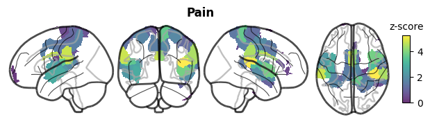
../_images/nb_introduction_intro07_visualization_22_1.png

[15]:

(<Figure size 720x180 with 6 Axes>, [<Axes: >])

[16]:

# plot multiple X maps with a shared color scale
nsp_pain.plot_brain(
    data="X",
    maps=["VAChT", "NET", "KOR"],  # only these three
    shared_colorscale=True,
    ncols=3,
    symmetric_cmap=False
)

WARNING | 20/07/26 18:22:13 | nispace.plotting: Brain plotting in NiSpace is experimental. If things look off, feel free to raise a GitHub issue!
INFO | 20/07/26 18:22:13 | nispace.plotting: brainplot: threshold='auto' → 0.0001124086047639139
INFO | 20/07/26 18:22:13 | nispace.plotting: brainplot: kind='glass', img_mode='None', surf_space='None', mni_space='MNI152NLin2009cAsym', surf_mesh='inflated'

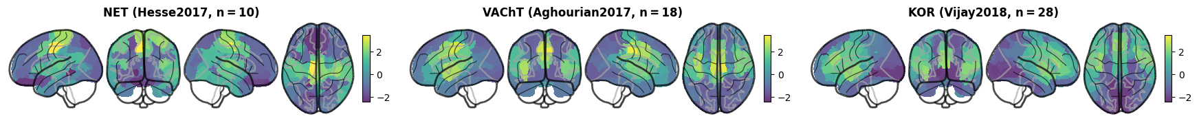
../_images/nb_introduction_intro07_visualization_23_1.png

[16]:

(<Figure size 2160x180 with 18 Axes>, [<Axes: >, <Axes: >, <Axes: >])

Surface mesh options

[17]:

# pial surface instead of inflated
nsp_pain.plot_brain(data="Y", surf_mesh="pial")

WARNING | 20/07/26 18:22:24 | nispace.plotting: Brain plotting in NiSpace is experimental. If things look off, feel free to raise a GitHub issue!
INFO | 20/07/26 18:22:24 | nispace.plotting: brainplot: threshold='auto' → 0.0017398296622559428
INFO | 20/07/26 18:22:24 | nispace.plotting: brainplot: kind='glass', img_mode='None', surf_space='None', mni_space='MNI152NLin2009cAsym', surf_mesh='pial'

../_images/nb_introduction_intro07_visualization_25_1.png

[17]:

(<Figure size 720x180 with 6 Axes>, [<Axes: >])

Summary

``nsp.plot()`` key arguments:

Argument	Options	Effect
`values`	`"coloc"`, `"z"`, `"p"`	What to show on x-axis
`mc_method`	`"meff"`, `"fdr_bh"`, `"bonferroni"`, `"maxT"`, …	Multiple comparison correction
`sort_by`	`"coloc"`, `"p"`, `"set"`	Bar ordering
`annot_p`	`"right"`, `"both"`, `False`	Significance markers
`X_maps`	list of strings	Select subset of reference maps
`ax`	matplotlib Axes	Embed in existing figure

``nsp.plot_brain()`` key arguments:

Argument	Options	Effect
`data`	`"Y"`, `"X"`, DataFrame	Which maps to render
`maps`	string or list	Select subset of maps
`kind`	`"surface"`, `"glass"`, `"slice"`	Rendering mode
`cmap`	any matplotlib colormap	Colormap
`symmetric_cmap`	bool	Zero-centered color scale
`shared_colorscale`	bool	Same scale across all maps

Next: Notebook 8 covers the standalone brainplot() function — useful whenever you want to visualize brain maps outside of a NiSpace analysis.