Working with imaging phenotypes (Y data)

In real neuroimaging studies, you rarely have a single group-average brain map ready to go. More often you have individual subject images that you need to transform into a group-level phenotype before you can run a colocalization.

This notebook covers:

Computing group-level effect sizes with transform_y() (Hedges’ g, Cohen’s d, z-scores, percentiles)
Removing confounding effects with clean_y() (covariate regression, ComBat harmonization)

We use the "anorexianervosa" example dataset: 50 patients and 50 healthy controls with parcellated grey matter values.

Note: This dataset is simulated and not intended for scientific use. The numbers are realistic but fabricated — do not draw any clinical or scientific conclusions from it.

[1]:

import tqdm.notebook
tqdm.notebook.tqdm = tqdm.tqdm

import numpy as np
import pandas as pd

Load the example dataset

The anorexia nervosa example dataset contains parcellated grey matter maps for 100 subjects. The group labels are encoded in the subject IDs.

[2]:

from nispace.datasets import fetch_example, fetch_reference

# load individual subject data
an_data = fetch_example("anorexianervosa", parcellation="Schaefer200")

# extract group labels from subject IDs
groups = an_data.index.str.extract(r'(AN|HC)$')[0].values

print(f"Data: {an_data.shape[0]} subjects x {an_data.shape[1]} parcels")
print(f"Groups: {pd.Series(groups).value_counts().to_dict()}")
an_data.head(3)

INFO | 01/06/26 15:03:25 | nispace.datasets: Loading example dataset: 'anorexianervosa', parcellated with: Schaefer200Parcels7Networks.
Data: 100 subjects x 200 parcels
Groups: {'AN': 50, 'HC': 50}

[2]:

	hemi-L_div-Vis_lab-1	hemi-L_div-Vis_lab-2	hemi-L_div-Vis_lab-3	hemi-L_div-Vis_lab-4	hemi-L_div-Vis_lab-5	hemi-L_div-Vis_lab-6	hemi-L_div-Vis_lab-7	hemi-L_div-Vis_lab-8	hemi-L_div-Vis_lab-9	hemi-L_div-Vis_lab-10	...	hemi-R_div-Default_lab-PFCm+1	hemi-R_div-Default_lab-PFCm+2	hemi-R_div-Default_lab-PFCm+3	hemi-R_div-Default_lab-PFCm+4	hemi-R_div-Default_lab-PFCm+5	hemi-R_div-Default_lab-PFCm+6	hemi-R_div-Default_lab-PFCm+7	hemi-R_div-Default_lab-PCC+1	hemi-R_div-Default_lab-PCC+2	hemi-R_div-Default_lab-PCC+3
sub-001AN	0.607015	0.666528	0.688496	0.334800	0.329322	0.562516	0.451181	0.573052	0.401972	0.672295	...	0.650113	0.603506	0.630403	0.408940	0.371325	0.644625	0.484537	0.658464	0.627889	0.632716
sub-002AN	0.788824	0.554837	0.647586	0.499502	0.445121	0.631092	0.287457	0.448134	0.340598	0.358523	...	0.845582	0.479605	0.362507	0.475748	0.407921	0.661211	0.546743	0.485640	0.694245	0.543393
sub-003AN	0.735806	0.709086	0.696516	0.500039	0.323851	0.514095	0.494061	0.544062	0.418107	0.600964	...	0.792297	0.628415	0.523004	0.585326	0.463725	0.587687	0.596047	0.645918	0.566473	0.550393

3 rows × 200 columns

Setting up NiSpace with individual subject data

When y is a DataFrame with one row per subject, NiSpace treats it as individual-level data. We pass the group vector separately when we call transform_y().

We also load the PET reference data.

[3]:

from nispace.api import NiSpace

pet_maps = fetch_reference("pet", parcellation="Schaefer200",
                           collection="UniqueTracers", print_references=False)

nsp = NiSpace(
    x=pet_maps,
    y=an_data,         # individual subject maps — one row per subject
    parcellation="Schaefer200",
    n_proc=4,
    seed=42
)
nsp.fit()
print(f"Fitted. Y shape: {nsp.get_y().shape}")

INFO | 01/06/26 15:03:25 | nispace.datasets: Loading pet maps.
INFO | 01/06/26 15:03:25 | nispace.datasets: Loading integrated collection 'UniqueTracers' for dataset 'pet'.
INFO | 01/06/26 15:03:25 | nispace.datasets: Filtering maps by collection.
INFO | 01/06/26 15:03:25 | nispace.datasets: Loading data parcellated with 'Schaefer200Parcels7Networks'
INFO | 01/06/26 15:03:25 | nispace.api: *** NiSpace.fit() - Data extraction and preparation. ***
INFO | 01/06/26 15:03:25 | nispace.core.parcellation: Building multi-space Parcellation for 'Schaefer200Parcels7Networks' from library.
INFO | 01/06/26 15:03:25 | nispace.core.parcellation: Available spaces: MNI152NLin2009cAsym, MNI152NLin6Asym, fsaverage, fsLR
INFO | 01/06/26 15:03:25 | nispace.core.parcellation: Parcellation 'Schaefer200Parcels7Networks': validation passed.
INFO | 01/06/26 15:03:25 | nispace.api: Checking input data for 'x' (should be, e.g., PET data):
INFO | 01/06/26 15:03:25 | nispace.io: Input type: DataFrame, assuming parcellated data with shape (n_files/subjects/etc, n_parcels).
WARNING | 01/06/26 15:03:25 | nispace.io: Parcellated data contains nan values!
INFO | 01/06/26 15:03:25 | nispace.api: Got 'x' data for 29 x 200 parcels.
INFO | 01/06/26 15:03:25 | nispace.api: Checking input data for 'y' (should be, e.g., subject data):
INFO | 01/06/26 15:03:25 | nispace.io: Input type: DataFrame, assuming parcellated data with shape (n_files/subjects/etc, n_parcels).
INFO | 01/06/26 15:03:25 | nispace.api: Got 'y' data for 100 x 200 parcels.
INFO | 01/06/26 15:03:25 | nispace.api: Z-standardizing 'X' data.
INFO | 01/06/26 15:03:25 | nispace.api: Returning Y dataframe:
| Y_TRANSFORM |
| False       | 
Fitted. Y shape: (100, 200)

Computing group-level effect sizes with `transform_y()`

To run a spatial colocalization, we need a single group-level map. transform_y() computes this for us, using a formula that specifies the comparison.

The group vector tells NiSpace which subjects belong to which group. The convention is that group “a” (here: AN) is compared against group “b” (here: HC).

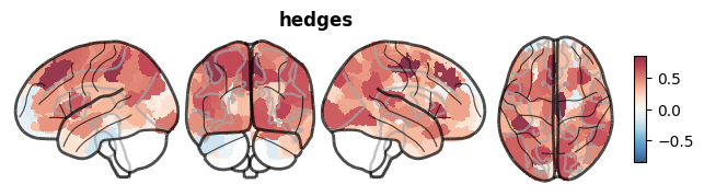
Hedges’ g

Hedges’ g is a bias-corrected version of Cohen’s d — the most common effect size metric for group comparisons. A negative g at a given parcel means the AN group has lower grey matter there compared to controls.

[4]:

# compute Hedges' g: AN vs. HC
# the formula "hedges(a,b)" computes Hedges' g for group a (AN) vs. group b (HC)
nsp.transform_y(
    transform="hedges(a,b)",
    groups=groups  # vector of group labels, same length as number of subjects
)

hedges_g = nsp.get_y()
print(f"After transform_y: {hedges_g.shape}  (one row = one group comparison)")
print(f"Value range: [{hedges_g.values.min():.2f}, {hedges_g.values.max():.2f}]")
hedges_g

INFO | 01/06/26 15:03:25 | nispace.api: *** NiSpace.transform_y() - Y transformation and comparison. ***
INFO | 01/06/26 15:03:25 | nispace.api: Groups/sessions vector provided, ensuring dummy-coding.
INFO | 01/06/26 15:03:25 | nispace.api: Applying Y transform 'hedges(a,b)'.
INFO | 01/06/26 15:03:26 | nispace.api: Returning Y dataframe:
| Y_TRANSFORM |
| hedges(a,b) | 
After transform_y: (1, 200)  (one row = one group comparison)
Value range: [-0.24, 0.86]

[4]:

	hemi-L_div-Vis_lab-1	hemi-L_div-Vis_lab-2	hemi-L_div-Vis_lab-3	hemi-L_div-Vis_lab-4	hemi-L_div-Vis_lab-5	hemi-L_div-Vis_lab-6	hemi-L_div-Vis_lab-7	hemi-L_div-Vis_lab-8	hemi-L_div-Vis_lab-9	hemi-L_div-Vis_lab-10	...	hemi-R_div-Default_lab-PFCm+1	hemi-R_div-Default_lab-PFCm+2	hemi-R_div-Default_lab-PFCm+3	hemi-R_div-Default_lab-PFCm+4	hemi-R_div-Default_lab-PFCm+5	hemi-R_div-Default_lab-PFCm+6	hemi-R_div-Default_lab-PFCm+7	hemi-R_div-Default_lab-PCC+1	hemi-R_div-Default_lab-PCC+2	hemi-R_div-Default_lab-PCC+3
hedges	0.234659	0.056813	0.107451	0.05087	0.536093	0.22262	0.138825	0.136664	0.175492	0.046341	...	0.10195	-0.240146	-0.14014	-0.03309	-0.058849	-0.164091	0.003687	0.119205	0.403226	0.416562

1 rows × 200 columns

[5]:

# visualize on the brain
nsp.plot_brain(data="Y", symmetric_cmap=True)

INFO | 01/06/26 15:03:26 | nispace.api: *** NiSpace.plot_brain() ***
INFO | 01/06/26 15:03:26 | nispace.api: Plotting Y data (Y_transform='hedges(a,b)').
INFO | 01/06/26 15:03:26 | nispace.api: Returning Y dataframe:
| Y_TRANSFORM |
| hedges(a,b) | 
WARNING | 01/06/26 15:03:26 | nispace.plotting: Brain plotting in NiSpace is experimental. If things look off, feel free to raise a GitHub issue!
INFO | 01/06/26 15:03:26 | nispace.plotting: brainplot: threshold='auto' → 0.0009347720188088715
INFO | 01/06/26 15:03:26 | nispace.core.parcellation: Lazy-loading parcellation image for space 'MNI152NLin2009cAsym'.
INFO | 01/06/26 15:03:26 | nispace.core.parcellation: Parcellation 'Schaefer200Parcels7Networks': active space set to 'MNI152NLin2009cAsym'.
INFO | 01/06/26 15:03:26 | nispace.plotting: brainplot: kind='glass', img_mode='None', surf_space='None', mni_space='MNI152NLin2009cAsym', surf_mesh='inflated'

../_images/nb_introduction_intro04_imaging_phenotypes_8_1.png

[5]:

(<Figure size 720x180 with 6 Axes>, [<Axes: >])

Widespread negative values are expected: anorexia nervosa is associated with global grey matter reductions, most pronounced in frontal and temporal regions.

Cohen’s d

Cohen’s d is the non-bias-corrected version. With n=50 per group the difference from Hedges’ g is minimal, but it’s good to know both are available.

[6]:

nsp.transform_y(transform="cohen(a,b)", groups=groups)
cohens_d = nsp.get_y()
print(f"Cohen's d range: [{cohens_d.values.min():.2f}, {cohens_d.values.max():.2f}]")

INFO | 01/06/26 15:03:29 | nispace.api: *** NiSpace.transform_y() - Y transformation and comparison. ***
INFO | 01/06/26 15:03:29 | nispace.api: Groups/sessions vector provided, ensuring dummy-coding.
INFO | 01/06/26 15:03:29 | nispace.api: Applying Y transform 'cohen(a,b)'.
INFO | 01/06/26 15:03:29 | nispace.api: Returning Y dataframe:
| Y_TRANSFORM |
| cohen(a,b)  | 
Cohen's d range: [-0.24, 0.87]

Z-scores (individual deviation maps)

Instead of a single group map, we can compute a deviation map for each patient: how many standard deviations does this individual deviate from the control mean at each parcel? This is useful for individual-level analyses — see Notebook 11.

[7]:

# z-score: each AN subject mapped relative to HC mean and SD
nsp.transform_y(transform="zscore(a,b)", groups=groups)

zscores = nsp.get_y()
print(f"Z-score maps: {zscores.shape}  (one row per AN subject)")
zscores.head(3)

INFO | 01/06/26 15:03:29 | nispace.api: *** NiSpace.transform_y() - Y transformation and comparison. ***
INFO | 01/06/26 15:03:29 | nispace.api: Groups/sessions vector provided, ensuring dummy-coding.
INFO | 01/06/26 15:03:29 | nispace.api: Applying Y transform 'zscore(a,b)'.
INFO | 01/06/26 15:03:29 | nispace.api: Returning Y dataframe:
| Y_TRANSFORM |
| zscore(a,b) | 
Z-score maps: (50, 200)  (one row per AN subject)

[7]:

	hemi-L_div-Vis_lab-1	hemi-L_div-Vis_lab-2	hemi-L_div-Vis_lab-3	hemi-L_div-Vis_lab-4	hemi-L_div-Vis_lab-5	hemi-L_div-Vis_lab-6	hemi-L_div-Vis_lab-7	hemi-L_div-Vis_lab-8	hemi-L_div-Vis_lab-9	hemi-L_div-Vis_lab-10	...	hemi-R_div-Default_lab-PFCm+1	hemi-R_div-Default_lab-PFCm+2	hemi-R_div-Default_lab-PFCm+3	hemi-R_div-Default_lab-PFCm+4	hemi-R_div-Default_lab-PFCm+5	hemi-R_div-Default_lab-PFCm+6	hemi-R_div-Default_lab-PFCm+7	hemi-R_div-Default_lab-PCC+1	hemi-R_div-Default_lab-PCC+2	hemi-R_div-Default_lab-PCC+3
sub-001AN	-0.917006	1.000070	1.132374	-1.605360	-0.771186	0.379098	-0.077323	0.378764	-0.604761	1.196448	...	-0.254770	-0.552606	1.362208	-0.933297	-0.946297	0.840285	-0.186260	0.167540	0.128992	0.551934
sub-002AN	1.005458	-0.029039	0.710286	0.111984	0.356170	1.074949	-1.508936	-0.839125	-1.304369	-2.243848	...	1.885931	-1.872780	-1.198049	-0.258558	-0.572263	1.023198	0.488698	-1.701267	0.837380	-0.358096
sub-003AN	0.444845	1.392190	1.215116	0.117580	-0.824451	-0.112243	0.297631	0.096133	-0.420842	0.414352	...	1.302371	-0.287197	0.335808	0.848146	-0.001928	0.212359	1.023656	0.031869	-0.526657	-0.286777

3 rows × 200 columns

For colocalization analyses, we typically average across subjects to get one group-level map. The Hedges’ g approach does this in one step. But for individual-level colocalization you’d keep all rows and analyze them separately.

Removing confounds with `clean_y()`

Grey matter maps are affected by confounds that have nothing to do with the disorder: age, sex, total intracranial volume, and scanner site are the usual suspects. clean_y() lets you regress these out before running colocalization.

NiSpace distinguishes between two types of regression:

“within”: regression across parcels within each map (e.g., regressing out a whole-brain grey matter map to control for global effects)
“between”: regression across subjects (e.g., removing age or sex effects)

Let’s generate a synthetic age vector for demonstration and show how to regress it out.

[8]:

# reset to individual subject data for this demo
nsp_clean = NiSpace(
    x=pet_maps,
    y=an_data,
    parcellation="Schaefer200",
    seed=42
)
nsp_clean.fit()

# generate a synthetic age vector: AN mean=25, HC mean=30, SD=5 for both
# (realistic for this kind of study)
rng = np.random.default_rng(42)
age_AN = rng.normal(25, 5, 50)
age_HC = rng.normal(30, 5, 50)
age = np.concatenate([age_AN, age_HC])

# sex: roughly balanced (0=male, 1=female), NiSpace treats string covariates automatically as categorical
sex = rng.permutation(["f"]*80 + ["m"]*20)

print(f"Age: mean={age.mean():.1f}, SD={age.std():.1f}")
print(f"Sex: {(sex=='f').sum()} female, {(sex=='m').sum()} male")

INFO | 01/06/26 15:03:29 | nispace.api: *** NiSpace.fit() - Data extraction and preparation. ***
INFO | 01/06/26 15:03:29 | nispace.core.parcellation: Building multi-space Parcellation for 'Schaefer200Parcels7Networks' from library.
INFO | 01/06/26 15:03:29 | nispace.core.parcellation: Available spaces: MNI152NLin2009cAsym, MNI152NLin6Asym, fsaverage, fsLR
INFO | 01/06/26 15:03:29 | nispace.core.parcellation: Parcellation 'Schaefer200Parcels7Networks': validation passed.
INFO | 01/06/26 15:03:29 | nispace.api: Checking input data for 'x' (should be, e.g., PET data):
INFO | 01/06/26 15:03:29 | nispace.io: Input type: DataFrame, assuming parcellated data with shape (n_files/subjects/etc, n_parcels).
WARNING | 01/06/26 15:03:29 | nispace.io: Parcellated data contains nan values!
INFO | 01/06/26 15:03:29 | nispace.api: Got 'x' data for 29 x 200 parcels.
INFO | 01/06/26 15:03:29 | nispace.api: Checking input data for 'y' (should be, e.g., subject data):
INFO | 01/06/26 15:03:29 | nispace.io: Input type: DataFrame, assuming parcellated data with shape (n_files/subjects/etc, n_parcels).
INFO | 01/06/26 15:03:29 | nispace.api: Got 'y' data for 100 x 200 parcels.
INFO | 01/06/26 15:03:29 | nispace.api: Z-standardizing 'X' data.
Age: mean=27.2, SD=4.2
Sex: 80 female, 20 male

[9]:

# regress age and sex out from the individual subject maps
# how="between" means: regression across subjects
# covariates_between is a DataFrame with one row per subject
covariates = pd.DataFrame({"age": age, "sex": sex}, index=an_data.index)

nsp_clean.clean_y(
    how="between",
    covariates_between=covariates
)

print("Covariate regression done.")
print(f"Y shape after cleaning: {nsp_clean.get_y().shape}")

INFO | 01/06/26 15:03:29 | nispace.api: *** NiSpace.clean_y() - Y covariate regression. ***
INFO | 01/06/26 15:03:29 | nispace.api: Performing covariate regression between maps/subjects (e.g., age, sex, site).
INFO | 01/06/26 15:03:29 | nispace.core.clean_y: Detected categorical covariates: ['sex']; continuous: ['age'].
INFO | 01/06/26 15:03:29 | nispace.core.clean_y: Regressing 2 between covariate(s) from Y.

Regressing 2 between covariate(s) from Y (1 proc): 100%|██████████████████████████████████████████████████████████████████████████████████████████| 200/200 [00:00<00:00, 14376.12it/s]

Covariate regression done.
INFO | 01/06/26 15:03:29 | nispace.api: Returning Y dataframe:
| Y_TRANSFORM |
| False       | 
Y shape after cleaning: (100, 200)

After cleaning, we can compute effect sizes on the covariate-corrected maps:

[10]:

nsp_clean.transform_y(transform="hedges(a,b)", groups=groups)
hedges_g_clean = nsp_clean.get_y()

print(f"Hedges' g after covariate regression: range [{hedges_g_clean.values.min():.2f}, {hedges_g_clean.values.max():.2f}]")

INFO | 01/06/26 15:03:29 | nispace.api: *** NiSpace.transform_y() - Y transformation and comparison. ***
INFO | 01/06/26 15:03:29 | nispace.api: Groups/sessions vector provided, ensuring dummy-coding.
INFO | 01/06/26 15:03:29 | nispace.api: Applying Y transform 'hedges(a,b)'.
INFO | 01/06/26 15:03:29 | nispace.api: Returning Y dataframe:
| Y_TRANSFORM |
| hedges(a,b) | 
Hedges' g after covariate regression: range [-0.34, 0.69]

ComBat harmonization

If your data comes from multiple scanners or study sites, clean_y() also supports ComBat harmonization (a Bayesian framework for removing scanner effects while preserving biological variability). Pass combat=True and include a "site" column in your covariates DataFrame:

covariates_with_site = pd.DataFrame({
    "age": age,
    "sex": sex,
    "site": site_labels  # scanner/site identifier per subject
}, index=an_data.index)

nsp_clean.clean_y(
    how="between",
    covariates_between=covariates_with_site,
    combat=True
)

ComBat removes site effects while keeping the biological covariates (age, sex) protected.

The full preprocessing pipeline

Putting it all together, a typical preprocessing pipeline before colocalization looks like this:

nsp = NiSpace(x=pet_maps, y=an_data, parcellation="Schaefer200")
nsp.fit()                                      # parcellate
nsp.clean_y(                                   # remove confounds
    how="between",
    covariates_between=covariates
)
nsp.transform_y(                               # compute effect sizes
    transform="hedges(a,b)",
    groups=groups
)
nsp.colocalize("spearman")                     # correlate with reference
nsp.permute("groups", n_perm=10000)            # permutation test (group labels)
nsp.plot()

Note that when group labels are permuted (permute("groups")), we permute the subject labels before computing the effect size — this gives a more principled null model than permuting the maps. This is covered in detail in Notebook 5.

Summary

Method	What it does
`transform_y("hedges(a,b)", groups=...)`	Hedges’ g per parcel (group a vs. b)
`transform_y("cohen(a,b)", groups=...)`	Cohen’s d per parcel
`transform_y("zscore(a,b)", groups=...)`	Z-score per subject (group a relative to b)
`clean_y(how="between", covariates_between=df)`	Regress out between-subject confounds
`clean_y(how="within", covariates_within=df)`	Regress out within-map confounds (e.g., grey matter)
`clean_y(..., combat=True)`	ComBat site harmonization

Next: Notebook 5 covers the null model methods in detail.