Advanced topics

This notebook covers advanced features of NiSpace:

Individual-level colocalization — compute colocalization for each subject separately.
Individual-level deviation colocalization — compute colocalization for each subject separately using z-score maps.
Dimensionality reduction (reduce_x()) — summarize a large set of reference maps into a smaller number of components before colocalization.
Alternative colocalization methods — partial correlation, PLS, ridge regression, and more.

We use the ENIGMA reference datasets (enigmathick and enigmaarea) as our input maps here — these contain published cortical thickness and surface area effect sizes (Cohen’s d) for many psychiatric disorders vs. healthy controls. Note that we’re using reference data as our input maps, which, in the case of ENIGMA maps, is however often done: it lets us ask questions like “which reference systems explain patterns of grey matter alterations across psychiatric disorders?”

[1]:

import tqdm.notebook
tqdm.notebook.tqdm = tqdm.tqdm

import numpy as np
import pandas as pd

[2]:

from nispace.datasets import fetch_reference, fetch_example
from nispace.api import NiSpace

# ENIGMA cortical thickness effect sizes (Cohen's d, cases vs. controls)
# These are reference datasets — we use them as target maps (Y) here
enigma_thick = fetch_reference("enigmathick", parcellation="DesikanKilliany", collection="Adult",
                               print_references=False)
print(f"ENIGMA thickness: {enigma_thick.shape[0]} disorders x {enigma_thick.shape[1]} cortical parcels")
print("Disorders:", list(enigma_thick.index))

# Continuous resting-state network (RSN) reference maps for colocalization
pet_maps = fetch_reference("rsn", parcellation="DesikanKilliany",
                           print_references=False)
print(f"PET: {pet_maps.shape[0]} maps x {pet_maps.shape[1]} parcels")

INFO | 01/06/26 15:07:43 | nispace.datasets: Loading enigmathick maps.
INFO | 01/06/26 15:07:43 | nispace.datasets: Loading integrated collection 'Adult' for dataset 'enigmathick'.
INFO | 01/06/26 15:07:43 | nispace.datasets: Filtering maps by collection.
INFO | 01/06/26 15:07:43 | nispace.datasets: Loading data parcellated with 'DesikanKilliany'
ENIGMA thickness: 17 disorders x 68 cortical parcels
Disorders: [('dx-mdd_age-adult_pub-schmaal2017',), ('dx-adhd_age-allages_pub-hoogman2019',), ('dx-adhd_age-adult_pub-hoogman2019',), ('dx-asd_pub-vanrooij2018',), ('dx-bd_age-adult_pub-hibar2018',), ('dx-scz_pub-vanerp2018',), ('dx-ocd_age-adult_pub-boedhoe2018',), ('dx-epilepsy_pub-whelan2018',), ('dx-epilepsy_subtype-gge_pub-whelan2018',), ('dx-epilepsy_subtype-ltle_pub-whelan2018',), ('dx-epilepsy_subtype-rtle_pub-whelan2018',), ('dx-22q_pub-sun2020',), ('dx-an_pub-walton2022',), ('dx-an_subtype-acAN_pub-walton2022',), ('dx-an_subtype-pwrAN_pub-walton2022',), ('dx-antisocial_pub-gao2024',), ('dx-pd_pub-laansma2021',)]
INFO | 01/06/26 15:07:43 | nispace.datasets: Loading rsn maps.
INFO | 01/06/26 15:07:43 | nispace.datasets: Loading data parcellated with 'DesikanKilliany'
PET: 14 maps x 68 parcels

Individual-level colocalization

The ENIGMA dataset gives us effect size maps for multiple disorders simultaneously. We can test all disorders at once by passing the full DataFrame as y.

[3]:

nsp = NiSpace(
    x=pet_maps,
    y=enigma_thick,   # all 22 disorder maps as input
    parcellation="DesikanKilliany",
    seed=42,
    n_proc=4
)
nsp.fit()
nsp.colocalize("spearman")
nsp.permute("maps", n_perm=1000)
nsp.correct_p()

colocs = nsp.get_colocalizations()
print(f"Result: {colocs.shape[0]} disorders x {colocs.shape[1]} receptors")
p_values = nsp.get_p_values()
print(f"Result: {p_values.shape[0]} x {p_values.shape[1]} receptors")

INFO | 01/06/26 15:07:43 | nispace.api: *** NiSpace.fit() - Data extraction and preparation. ***
INFO | 01/06/26 15:07:43 | nispace.core.parcellation: Building multi-space Parcellation for 'DesikanKilliany' from library.
INFO | 01/06/26 15:07:43 | nispace.core.parcellation: Available spaces: MNI152NLin2009cAsym, MNI152NLin6Asym, fsaverage, fsLR
INFO | 01/06/26 15:07:43 | nispace.core.parcellation: Parcellation 'DesikanKilliany': validation passed.
INFO | 01/06/26 15:07:43 | nispace.api: Checking input data for 'x' (should be, e.g., PET data):
INFO | 01/06/26 15:07:43 | nispace.io: Input type: DataFrame, assuming parcellated data with shape (n_files/subjects/etc, n_parcels).
INFO | 01/06/26 15:07:43 | nispace.api: Got 'x' data for 14 x 68 parcels.
INFO | 01/06/26 15:07:43 | nispace.api: Checking input data for 'y' (should be, e.g., subject data):
INFO | 01/06/26 15:07:43 | nispace.io: Input type: DataFrame, assuming parcellated data with shape (n_files/subjects/etc, n_parcels).
WARNING | 01/06/26 15:07:43 | nispace.io: Parcellated data contains nan values!
INFO | 01/06/26 15:07:43 | nispace.api: Got 'y' data for 17 x 68 parcels.
INFO | 01/06/26 15:07:43 | nispace.api: Z-standardizing 'X' data.
INFO | 01/06/26 15:07:43 | nispace.api: *** NiSpace.colocalize() - Estimating X & Y colocalizations. ***
INFO | 01/06/26 15:07:43 | nispace.api: Running 'spearman' colocalization.
INFO | 01/06/26 15:07:43 | nispace.api: Pre-ranking X and Y data.

Colocalizing (spearman, 4 proc): 100%|█████████████████████████████████████████████████████████████████████████████████████████████████████████████████| 17/17 [00:03<00:00,  4.81it/s]

INFO | 01/06/26 15:07:47 | nispace.api: *** NiSpace.permute() - Estimate exact non-parametric p values. ***
INFO | 01/06/26 15:07:47 | nispace.api: Permutation of: X maps.
INFO | 01/06/26 15:07:47 | nispace.api: Using default null method 'alexander_bloch' (parcellation null space: 'fsLR').
INFO | 01/06/26 15:07:47 | nispace.core.parcellation: Lazy-loading parcellation image for space 'fsLR'.
INFO | 01/06/26 15:07:47 | nispace.api: Will calculate p values for mean colocalization across Y maps. Set 'pooled_p=False' to compute p values for each Y map individually.
INFO | 01/06/26 15:07:47 | nispace.api: Loading observed colocalizations (method = 'spearman').
INFO | 01/06/26 15:07:47 | nispace.core.permute: No null maps found.
INFO | 01/06/26 15:07:47 | nispace.core.permute: Generating null maps (n = 1000, null_method = 'alexander_bloch').
INFO | 01/06/26 15:07:47 | nispace.nulls: Null map generation: Assuming n = 14 data vector(s) for n = 68 parcels.
INFO | 01/06/26 15:07:47 | nispace.nulls: Using provided precomputed spin matrix.


Spin null maps: 100%|█████████████████████████████████████████████████████████████████████████████████████████████████████████████████████████████████| 14/14 [00:00<00:00, 229.93it/s]

INFO | 01/06/26 15:07:47 | nispace.nulls: Null data generation finished.
INFO | 01/06/26 15:07:47 | nispace.core.permute: Z-standardizing null maps.


Processing null arrays (4 proc): 100%|███████████████████████████████████████████████████████████████████████████████████████████████████████████| 1000/1000 [00:00<00:00, 1000.44it/s]
Null colocalizations (spearman, 4 proc): 100%|███████████████████████████████████████████████████████████████████████████████████████████████████| 1000/1000 [00:00<00:00, 8190.83it/s]

INFO | 01/06/26 15:07:48 | nispace.core.permute: Calculating exact p-values (tails = {'rho': 'two'}).
Result: 17 disorders x 14 receptors
Result: 1 x 14 receptors

If we plot these data now with the automated method, what was bars before are now scatter points. Each point represents one ENIGMA cortical effect size map, respectively the disorder map’s association to each reference map.

We, by default calculate only one p value for the group-average, which here tests if there is a spatial pattern consistenly associated with ENIGMA maps across disorders.

[4]:

# plot all disorders
nsp.plot(sort_by="p")

INFO | 01/06/26 15:07:48 | nispace.plotting: Significance annotation: 2/14 p_uncorrected < 0.05, 1/14 p_meffgalwey < 0.05

../_images/nb_introduction_intro11_advanced_6_1.png

[4]:

(<Figure size 500x430 with 1 Axes>,
 <Axes: title={'center': "$Spearman's\\ Rho$ colocalization\n(permutation of $X\\ maps$)"}, xlabel='$Rho$'>,
 <seaborn._core.plot.Plotter at 0x16addc640>)

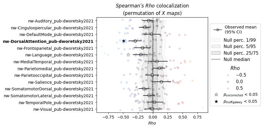
That is interesting in itself. But we might now want to know how each individual ENIGMA map colocalizes with each individual resting-state network.

To achieve that, we can set a flag in NiSpace.permute(), which deactivates the group-level p value computation.

[5]:

nsp.colocalize("spearman")
nsp.permute("maps", n_perm=1000, p_from_average_y_coloc=False)
nsp.correct_p()

# both the colocalization and the p value dataframes will now be a n_reference x n_enigma dataframe
colocs = nsp.get_colocalizations()
print(f"Colocalizations: {colocs.shape[0]} disorders x {colocs.shape[1]} receptors")
p_values = nsp.get_p_values()
pc_values = nsp.get_corrected_p_values()
print(f"P-Values: {p_values.shape[0]} disorders x {p_values.shape[1]} receptors")

Colocalizing (spearman, 4 proc): 100%|███████████████████████████████████████████████████████████████████████████████████████████████████████████████| 17/17 [00:00<00:00, 1535.42it/s]

INFO | 01/06/26 15:07:48 | nispace.core.permute: Found existing null maps.
INFO | 01/06/26 15:07:48 | nispace.core.permute: Z-standardizing null maps.


Processing null arrays (4 proc): 100%|███████████████████████████████████████████████████████████████████████████████████████████████████████████| 1000/1000 [00:00<00:00, 9310.72it/s]
Null colocalizations (spearman, 4 proc): 100%|███████████████████████████████████████████████████████████████████████████████████████████████████| 1000/1000 [00:00<00:00, 8353.24it/s]

INFO | 01/06/26 15:07:49 | nispace.core.permute: Calculating exact p-values (tails = {'rho': 'two'}).
Colocalizations: 17 disorders x 14 receptors
P-Values: 17 disorders x 14 receptors

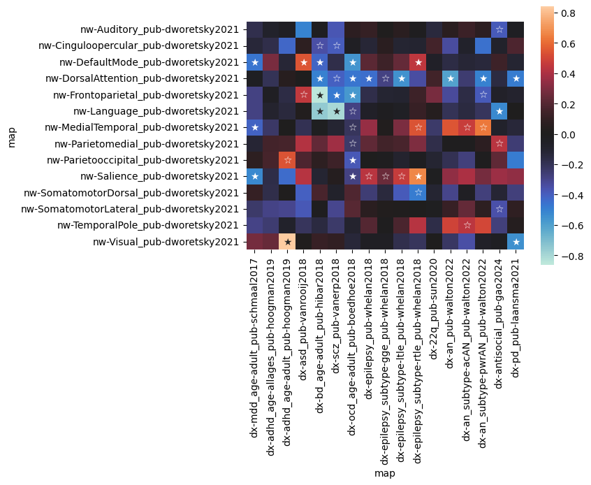
A heatmap is a typical means to visualize this. For now, we just use seaborn.heatmap() and add the p values as annotation.

[6]:

import seaborn as sns

sns.heatmap(
    colocs.T,
    center=0,
    square=True,
    annot=((p_values.T < 0.05).astype(int) + (pc_values.T.astype(int) < 0.05)) \
        .replace({0: "", 1: "☆", 2: "★"}),
    fmt="s"
)

[6]:

<Axes: xlabel='map', ylabel='map'>

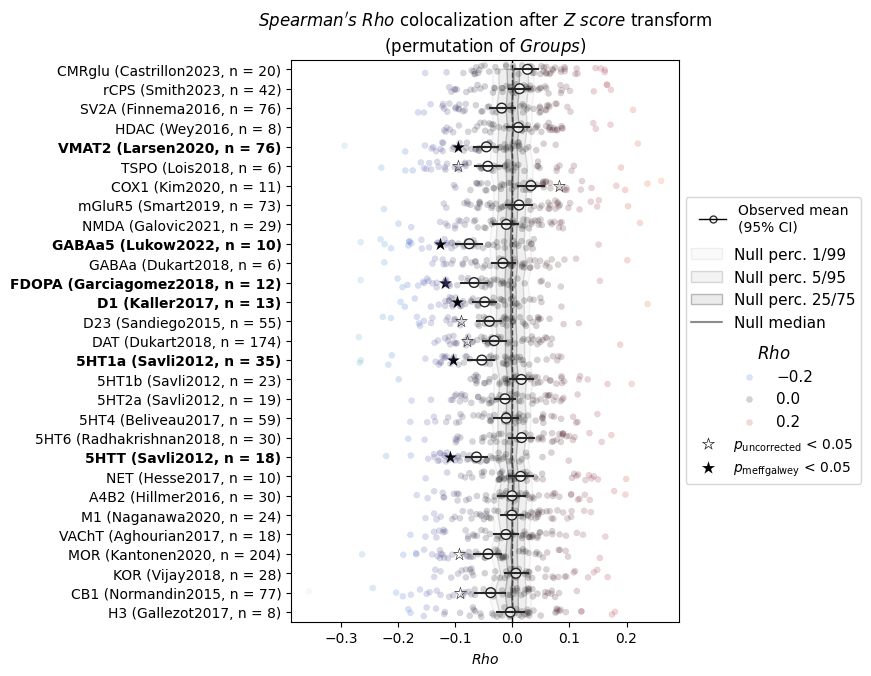
../_images/nb_introduction_intro11_advanced_10_1.png

Individual-level deviation colocalization

Except for the last, the analyses so far have produced group-level results: one colocalization value per disorder or condition. But we often may want to compute colocalization for each subject individually.

The "zscore(a,b)" transform in transform_y() produces one deviation map per subject in group A (patients). We can then colocalize each map separately and look at the distribution across subjects.

This is particularly useful for stratifying patients by their colocalization profile (e.g., identifying subgroups with different neurotransmitter involvement).

We return to the anorexia nervosa example dataset here — as a reminder, it is simulated and not intended for scientific use.

[7]:

from nispace.datasets import fetch_example

an_data = fetch_example("anorexianervosa", parcellation="Schaefer200")
groups = an_data.index.str.extract(r'(AN|HC)$')[0].values

pet_s200 = fetch_reference("pet", parcellation="Schaefer200",
                           collection="UniqueTracers", print_references=False)

nsp_indiv = NiSpace(
    x=pet_s200,
    y=an_data,
    parcellation="Schaefer200",
    seed=42,
    n_proc=4
)
nsp_indiv.fit()

# compute z-scores: each AN patient mapped relative to HC mean and SD
nsp_indiv.transform_y("zscore(a,b)", groups=groups)

print(f"Individual z-score maps: {nsp_indiv.get_y().shape}")

INFO | 01/06/26 15:07:49 | nispace.datasets: Loading example dataset: 'anorexianervosa', parcellated with: Schaefer200Parcels7Networks.
INFO | 01/06/26 15:07:49 | nispace.datasets: Loading pet maps.
INFO | 01/06/26 15:07:49 | nispace.datasets: Loading integrated collection 'UniqueTracers' for dataset 'pet'.
INFO | 01/06/26 15:07:49 | nispace.datasets: Filtering maps by collection.
INFO | 01/06/26 15:07:49 | nispace.datasets: Loading data parcellated with 'Schaefer200Parcels7Networks'
INFO | 01/06/26 15:07:49 | nispace.core.parcellation: Building multi-space Parcellation for 'Schaefer200Parcels7Networks' from library.
INFO | 01/06/26 15:07:49 | nispace.core.parcellation: Available spaces: MNI152NLin2009cAsym, MNI152NLin6Asym, fsaverage, fsLR
INFO | 01/06/26 15:07:49 | nispace.core.parcellation: Parcellation 'Schaefer200Parcels7Networks': validation passed.
INFO | 01/06/26 15:07:49 | nispace.io: Input type: DataFrame, assuming parcellated data with shape (n_files/subjects/etc, n_parcels).
WARNING | 01/06/26 15:07:49 | nispace.io: Parcellated data contains nan values!
INFO | 01/06/26 15:07:49 | nispace.io: Input type: DataFrame, assuming parcellated data with shape (n_files/subjects/etc, n_parcels).
Individual z-score maps: (50, 200)

[8]:

# colocalize each subject's z-score map with PET maps
nsp_indiv.colocalize("spearman")

# result: one row per AN subject, one column per receptor
indiv_colocs = nsp_indiv.get_colocalizations()
print(f"Individual colocalizations: {indiv_colocs.shape}")
indiv_colocs.head(5)

Colocalizing (spearman, 4 proc): 100%|███████████████████████████████████████████████████████████████████████████████████████████████████████████████| 50/50 [00:00<00:00, 2738.83it/s]

Individual colocalizations: (50, 29)

[8]:

set	General					Immunity		Glutamate		GABA	...	Serotonin		Noradrenaline/Acetylcholine				Opioids/Endocannabinoids			Histamine
map	target-CMRglu_tracer-fdg_n-20_dx-hc_pub-castrillon2023	target-rCPS_tracer-leucine_n-42_dx-hc_pub-smith2023	target-SV2A_tracer-ucbj_n-76_dx-hc_pub-finnema2016	target-HDAC_tracer-martinostat_n-8_dx-hc_pub-wey2016	target-VMAT2_tracer-dtbz_n-76_dx-hc_pub-larsen2020	target-TSPO_tracer-pbr28_n-6_dx-hc_pub-lois2018	target-COX1_tracer-ps13_n-11_dx-hc_pub-kim2020	target-mGluR5_tracer-abp688_n-73_dx-hc_pub-smart2019	target-NMDA_tracer-ge179_n-29_dx-hc_pub-galovic2021	target-GABAa5_tracer-ro154513_n-10_dx-hc_pub-lukow2022	...	target-5HT6_tracer-gsk215083_n-30_dx-hc_pub-radhakrishnan2018	target-5HTT_tracer-dasb_n-18_dx-hc_pub-savli2012	target-NET_tracer-mrb_n-10_dx-hc_pub-hesse2017	target-A4B2_tracer-flubatine_n-30_dx-hc_pub-hillmer2016	target-M1_tracer-lsn3172176_n-24_dx-hc_pub-naganawa2020	target-VAChT_tracer-feobv_n-18_dx-hc_pub-aghourian2017	target-MOR_tracer-carfentanil_n-204_dx-hc_pub-kantonen2020	target-KOR_tracer-ly2795050_n-28_dx-hc_pub-vijay2018	target-CB1_tracer-omar_n-77_dx-hc_pub-normandin2015	target-H3_tracer-gsk189254_n-8_dx-hc_pub-gallezot2017
sub-001AN	0.017047	0.063481	0.077512	0.022713	0.000522	-0.051870	0.031316	0.148510	0.033367	0.015989	...	0.069499	-0.024101	0.138824	0.103126	0.079042	0.082800	0.028306	0.148780	0.002946	-0.026949
sub-002AN	0.050685	0.028544	0.049336	0.059077	0.010109	0.077949	-0.063088	0.063228	0.019509	0.024376	...	0.106034	-0.044316	0.008265	0.082261	0.089020	0.044310	0.047142	0.109717	0.062302	0.077379
sub-003AN	0.049166	0.004716	-0.015789	0.042196	-0.058407	-0.095477	0.023831	0.051145	-0.006990	-0.146041	...	-0.019279	-0.117699	0.021439	-0.075802	0.021563	-0.054418	-0.077310	-0.029879	-0.072018	0.011837
sub-004AN	-0.063293	-0.073066	-0.114253	-0.047778	-0.121368	-0.006215	-0.059130	-0.078576	-0.080251	-0.033082	...	0.032534	-0.075188	-0.018891	-0.018200	-0.073574	0.018696	0.053493	0.072137	0.081855	-0.017590
sub-005AN	-0.048554	-0.017159	-0.094473	-0.034040	-0.040044	-0.007892	-0.018086	-0.036658	-0.035953	-0.065498	...	-0.004646	-0.065861	-0.006555	-0.031980	-0.044842	-0.027111	-0.076432	0.027479	0.015603	0.016296

5 rows × 29 columns

[9]:

# for permutation testing with individual maps, we permute group labels
# p values are computed for the MEAN colocalization across subjects by default
#  -> compare to the section above
nsp_indiv.permute("groups", groups=groups, n_perm=1000)
nsp_indiv.correct_p()
p_indiv = nsp_indiv.get_p_values()

print(f"P-values shape: {p_indiv.shape}")
print(p_indiv.T.sort_values(by=p_indiv.index[0]).head(10))

INFO | 01/06/26 15:07:49 | nispace.core.parcellation: Lazy-loading parcellation image for space 'fsLR'.

Permuting groups (4 proc): 100%|███████████████████████████████████████████████████████████████████████████████████████████████████████████████| 1000/1000 [00:00<00:00, 868745.65it/s]
Null transformations (spearman, 4 proc): 100%|██████████████████████████████████████████████████████████████████████████████████████████████████| 1000/1000 [00:00<00:00, 14698.29it/s]
Processing null arrays (4 proc): 100%|███████████████████████████████████████████████████████████████████████████████████████████████████████████| 1000/1000 [00:00<00:00, 7053.77it/s]
Null colocalizations (spearman, 4 proc): 100%|████████████████████████████████████████████████████████████████████████████████████████████████████| 1000/1000 [00:01<00:00, 972.59it/s]

INFO | 01/06/26 15:07:51 | nispace.core.permute: Calculating exact p-values (tails = {'rho': 'two'}).
P-values shape: (1, 29)
                                                                              mean
set                      map
Serotonin                target-5HTT_tracer-dasb_n-18_dx-hc_pub-savli2012    0.001
                         target-5HT1a_tracer-way100635_n-35_dx-hc_pub-sa...  0.001
GABA                     target-GABAa5_tracer-ro154513_n-10_dx-hc_pub-lu...  0.001
Dopamine                 target-FDOPA_tracer-fluorodopa_n-12_dx-hc_pub-g...  0.001
General                  target-VMAT2_tracer-dtbz_n-76_dx-hc_pub-larsen2020  0.002
Dopamine                 target-D1_tracer-sch23390_n-13_dx-hc_pub-kaller...  0.002
Opioids/Endocannabinoids target-MOR_tracer-carfentanil_n-204_dx-hc_pub-k...  0.008
Immunity                 target-TSPO_tracer-pbr28_n-6_dx-hc_pub-lois2018     0.012
Dopamine                 target-D23_tracer-flb457_n-55_dx-hc_pub-sandieg...  0.012
Opioids/Endocannabinoids target-CB1_tracer-omar_n-77_dx-hc_pub-normandin...  0.034

[10]:

# plot
nsp_indiv.plot()

INFO | 01/06/26 15:07:52 | nispace.plotting: Significance annotation: 12/29 p_uncorrected < 0.05, 6/29 p_meffgalwey < 0.05

../_images/nb_introduction_intro11_advanced_15_1.png

[10]:

(<Figure size 500x730 with 1 Axes>,
 <Axes: title={'center': "$Spearman's\\ Rho$ colocalization after $Z\\ score$ transform\n(permutation of $Groups$)"}, xlabel='$Rho$'>,
 <seaborn._core.plot.Plotter at 0x16c59ac10>)

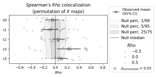
Dimensionality reduction with `reduce_x()`

When you have many reference maps (30 PET tracers, thousands of genes), interpreting individual colocalizations can be difficult — and many maps are correlated with each other. reduce_x() summarizes the reference maps into a smaller set of components using PCA, ICA, or factor analysis.

After reduction, colocalize() operates on the components instead of individual maps.

[11]:

# reduce the PET maps to their principal components
nsp.reduce_x("pca", n_components=5)  # keep 5 components

# colocalize on the reduced space
nsp.colocalize("spearman", X_reduction="pca")
nsp.permute("maps", n_perm=1000, X_reduction="pca")

pca_colocs = nsp.get_colocalizations(X_reduction="pca")
print(f"PCA colocalizations: {pca_colocs.shape[0]} disorders x {pca_colocs.shape[1]} components")
pca_colocs

INFO | 01/06/26 15:07:52 | nispace.core.reduce_x: Performing dimensionality reduction using pca (max components: 5, min EV: None).
INFO | 01/06/26 15:07:52 | nispace.core.reduce_x: Returning 5 principal component(s).

Colocalizing (spearman, 4 proc): 100%|███████████████████████████████████████████████████████████████████████████████████████████████████████████████| 17/17 [00:00<00:00, 1594.72it/s]

INFO | 01/06/26 15:07:52 | nispace.core.permute: Found existing null maps.
WARNING | 01/06/26 15:07:52 | nispace.core.permute: Not all X/Y variables in null maps. Will re-generate.
INFO | 01/06/26 15:07:52 | nispace.core.permute: Generating null maps (n = 1000, null_method = 'alexander_bloch').
INFO | 01/06/26 15:07:52 | nispace.nulls: Null map generation: Assuming n = 5 data vector(s) for n = 68 parcels.
INFO | 01/06/26 15:07:52 | nispace.nulls: Using provided precomputed spin matrix.


Spin null maps: 100%|███████████████████████████████████████████████████████████████████████████████████████████████████████████████████████████████████| 5/5 [00:00<00:00, 220.08it/s]

INFO | 01/06/26 15:07:52 | nispace.nulls: Null data generation finished.
INFO | 01/06/26 15:07:52 | nispace.core.permute: Z-standardizing null maps.


Processing null arrays (4 proc): 100%|███████████████████████████████████████████████████████████████████████████████████████████████████████████| 1000/1000 [00:00<00:00, 9487.83it/s]
Null colocalizations (spearman, 4 proc): 100%|██████████████████████████████████████████████████████████████████████████████████████████████████| 1000/1000 [00:00<00:00, 11323.65it/s]

INFO | 01/06/26 15:07:52 | nispace.core.permute: Calculating exact p-values (tails = {'rho': 'two'}).
PCA colocalizations: 17 disorders x 5 components

[11]:

	c0	c1	c2	c3	c4
map
dx-mdd_age-adult_pub-schmaal2017	0.350335	-0.381529	-0.178854	-0.356347	-0.011331
dx-adhd_age-allages_pub-hoogman2019	-0.132182	-0.057538	0.045820	-0.319895	0.396888
dx-adhd_age-adult_pub-hoogman2019	-0.014370	-0.526697	-0.062857	-0.445011	0.198560
dx-asd_pub-vanrooij2018	-0.310917	0.311928	0.475533	-0.249393	0.087193
dx-bd_age-adult_pub-hibar2018	0.180692	-0.700799	0.065560	0.539223	0.002533
dx-scz_pub-vanerp2018	-0.054100	-0.472228	0.179924	0.260594	-0.159836
dx-ocd_age-adult_pub-boedhoe2018	0.471912	-0.214527	-0.215989	0.270299	0.046994
dx-epilepsy_pub-whelan2018	-0.191002	0.080550	0.122663	0.522908	0.284856
dx-epilepsy_subtype-gge_pub-whelan2018	-0.044712	0.110665	0.224301	0.256793	0.414935
dx-epilepsy_subtype-ltle_pub-whelan2018	-0.248365	0.134195	0.039337	0.534235	0.306862
dx-epilepsy_subtype-rtle_pub-whelan2018	-0.472573	0.228192	0.047887	0.492719	0.115260
dx-22q_pub-sun2020	0.137077	0.161603	0.192222	-0.435269	-0.060933
dx-an_pub-walton2022	-0.162079	-0.120526	-0.237759	0.802155	0.065844
dx-an_subtype-acAN_pub-walton2022	-0.060853	0.031242	-0.094012	0.768742	-0.226304
dx-an_subtype-pwrAN_pub-walton2022	-0.221277	-0.236615	-0.235340	0.756421	0.055607
dx-antisocial_pub-gao2024	-0.104394	-0.192869	0.522142	0.132958	0.064234
dx-pd_pub-laansma2021	0.123394	0.376470	-0.037572	0.339391	0.208653

[12]:

nsp.plot(X_reduction="pca")

INFO | 01/06/26 15:07:53 | nispace.plotting: Significance annotation: 1/5 p_uncorrected < 0.05, 0/5 p_meffgalwey < 0.05 (no correction applied)

../_images/nb_introduction_intro11_advanced_18_1.png

[12]:

(<Figure size 500x250 with 1 Axes>,
 <Axes: title={'center': "$Spearman's\\ Rho$ colocalization\n(permutation of $X\\ maps$)"}, xlabel='$Rho$'>,
 <seaborn._core.plot.Plotter at 0x16e177e80>)

Alternative colocalization methods

Spearman correlation is the default, but NiSpace supports several other methods. Each has different assumptions and use cases.

Importantly, methods might return multiple different colocalization metrics. For example, a linear regression model ("mlr") already returns both beta coefficients (one for each X map, as for correlations) and the R^2 value (one across X maps). Each of these colocalization statistics will furthermore have an associated p values after .permute() has been run.

[13]:

# set up a simple analysis for comparison
nsp_methods = NiSpace(
    x=pet_maps,
    y=enigma_thick.loc[["dx-bd_age-adult_pub-hibar2018"]],  # just bipolar disorder for clarity
    parcellation="DesikanKilliany",
    seed=42
)
nsp_methods.fit()

# Pearson correlation
nsp_methods.colocalize("pearson")
pearson = nsp_methods.get_colocalizations()
print("Pearson:", pearson.values.squeeze())
print("")

# Multiple linear regression (MLR)
nsp_methods.colocalize("mlr")
mlr = nsp_methods.get_colocalizations()
print("MLR beta:", mlr["beta"].values.squeeze())
print("MLR R2:", mlr["r2"].values.squeeze())
print("")

# Partial least squares (PLS)
nsp_methods.colocalize("pls", n_components=3)
pls = nsp_methods.get_colocalizations()
print("PLS beta:", pls["beta"].values.squeeze())
print("PLS R2:", pls["r2"].values.squeeze())
print("")

# Dominance analysis (takes the longest)
nsp_methods.colocalize("dominance")
dom = nsp_methods.get_colocalizations()
print("Dominance: sum (matches MLR R2) :", dom["sum"].values.squeeze())
print("Dominance: total (sum of total is MLR R2):", dom["total"].values.squeeze())
print("Dominance: individual (like a leave-one-out MLR R2):", dom["individual"].values.squeeze())
print("Dominance: relative (fraction of sum R2):", dom["relative"].values.squeeze())

INFO | 01/06/26 15:07:53 | nispace.core.parcellation: Building multi-space Parcellation for 'DesikanKilliany' from library.
INFO | 01/06/26 15:07:53 | nispace.core.parcellation: Available spaces: MNI152NLin2009cAsym, MNI152NLin6Asym, fsaverage, fsLR
INFO | 01/06/26 15:07:53 | nispace.core.parcellation: Parcellation 'DesikanKilliany': validation passed.
INFO | 01/06/26 15:07:53 | nispace.io: Input type: DataFrame, assuming parcellated data with shape (n_files/subjects/etc, n_parcels).
INFO | 01/06/26 15:07:53 | nispace.io: Input type: DataFrame, assuming parcellated data with shape (n_files/subjects/etc, n_parcels).

Colocalizing (pearson, 1 proc): 100%|███████████████████████████████████████████████████████████████████████████████████████████████████████████████████| 1/1 [00:00<00:00, 311.80it/s]

Pearson: [ 0.09379738 -0.12041875 -0.32349086 -0.22995271 -0.70154136 -0.3893741
  0.25937384  0.10179116  0.20780352  0.17480677  0.14520817  0.13494447
  0.1137092   0.29869333]

Colocalizing (mlr, 1 proc): 100%|███████████████████████████████████████████████████████████████████████████████████████████████████████████████████████| 1/1 [00:00<00:00, 121.49it/s]

MLR beta: [ 0.00266048 -0.01679382 -0.02431268 -0.01540803 -0.02362837 -0.00963058
  0.00947228  0.00963644  0.00542823  0.02405527  0.00453575  0.00743604
  0.00379609  0.00881169]
MLR R2: 0.46437818

Colocalizing (pls, 1 proc): 100%|███████████████████████████████████████████████████████████████████████████████████████████████████████████████████████| 1/1 [00:00<00:00, 120.95it/s]

PLS beta: [ 0.0021201  -0.01162152 -0.01987142 -0.01660991 -0.024217   -0.00883197
  0.01095411  0.00524392  0.0065681   0.02115439  0.00681146  0.00787176
  0.00419393  0.01316884]
PLS R2: 0.5715146

Colocalizing (dominance, 1 proc): 100%|██████████████████████████████████████████████████████████████████████████████████████████████████████████████████| 1/1 [00:00<00:00,  3.70it/s]

Dominance: sum (matches MLR R2) : 0.46437818
Dominance: total (sum of total is MLR R2): [1.3349009e-04 8.5304175e-03 5.7703033e-02 3.6930375e-02 1.8202354e-01
 5.0407633e-02 2.7346514e-02 8.9180330e-04 1.0367648e-02 4.3500487e-02
 4.6723862e-03 1.7571739e-03 2.8868834e-04 3.9825007e-02]
Dominance: individual (like a leave-one-out MLR R2): [-0.00627205 -0.00057247  0.08408586  0.03669057  0.35684335  0.12443971
  0.05019241 -0.00470505  0.02745323  0.01524752  0.00595633  0.00311236
 -0.0021382   0.07029137]
Dominance: relative (fraction of sum R2): [2.87459872e-04 1.83695480e-02 1.24258704e-01 7.95264989e-02
 3.91972631e-01 1.08548664e-01 5.88884540e-02 1.92042463e-03
 2.23258715e-02 9.36746970e-02 1.00615975e-02 3.78392870e-03
 6.21666433e-04 8.57598558e-02]

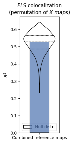
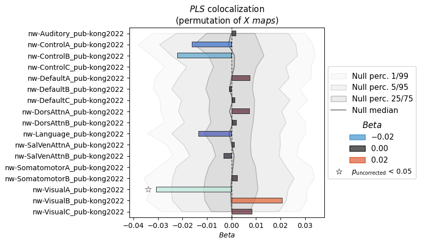
If we plot multi-outcome colocalization results, we will automatically get one plot for each metric. E.g., for the quite detailled dominance output:

[14]:

# first: run the proper permutation; will take some time for dominance analysis
nsp_methods.permute("maps", n_perm=1000, n_proc=4)
nsp_methods.correct_p()

# show
nsp_methods.plot()

INFO | 01/06/26 15:07:53 | nispace.core.parcellation: Lazy-loading parcellation image for space 'fsLR'.
INFO | 01/06/26 15:07:53 | nispace.core.permute: No null maps found.
INFO | 01/06/26 15:07:53 | nispace.core.permute: Generating null maps (n = 1000, null_method = 'alexander_bloch').
INFO | 01/06/26 15:07:53 | nispace.nulls: Null map generation: Assuming n = 14 data vector(s) for n = 68 parcels.
INFO | 01/06/26 15:07:53 | nispace.nulls: Using provided precomputed spin matrix.

Spin null maps: 100%|█████████████████████████████████████████████████████████████████████████████████████████████████████████████████████████████████| 14/14 [00:00<00:00, 257.90it/s]

INFO | 01/06/26 15:07:53 | nispace.nulls: Null data generation finished.
INFO | 01/06/26 15:07:53 | nispace.core.permute: Z-standardizing null maps.


Null colocalizations (dominance, 4 proc): 100%|████████████████████████████████████████████████████████████████████████████████████████████████████| 1000/1000 [01:03<00:00, 15.80it/s]

INFO | 01/06/26 15:08:57 | nispace.core.permute: Calculating exact p-values (tails = {'sum': 'upper', 'total': 'upper', 'individual': 'upper', 'relative': 'upper'}).
INFO | 01/06/26 15:08:57 | nispace.plotting: Significance annotation: 0/1 p_uncorrected < 0.05, 0/1 p_meffgalwey < 0.05

../_images/nb_introduction_intro11_advanced_22_5.png

INFO | 01/06/26 15:08:57 | nispace.plotting: Significance annotation: 1/14 p_uncorrected < 0.05, 1/14 p_meffgalwey < 0.05

../_images/nb_introduction_intro11_advanced_22_7.png

INFO | 01/06/26 15:08:57 | nispace.plotting: Significance annotation: 2/14 p_uncorrected < 0.05, 1/14 p_meffgalwey < 0.05

../_images/nb_introduction_intro11_advanced_22_9.png

INFO | 01/06/26 15:08:58 | nispace.plotting: Significance annotation: 0/14 p_uncorrected < 0.05, 0/14 p_meffgalwey < 0.05

../_images/nb_introduction_intro11_advanced_22_11.png

[14]:

{'sum': (<Figure size 170x500 with 1 Axes>,
  <Axes: title={'center': '$Dominance\\ Analysis$ colocalization\n(permutation of $X\\ maps$)'}, ylabel='$sum$'>,
  <seaborn._core.plot.Plotter at 0x168af05b0>),
 'total': (<Figure size 500x430 with 1 Axes>,
  <Axes: title={'center': '$Dominance\\ Analysis$ colocalization\n(permutation of $X\\ maps$)'}, xlabel='$Total\\ R^2$'>,
  <seaborn._core.plot.Plotter at 0x17acf1940>),
 'individual': (<Figure size 500x430 with 1 Axes>,
  <Axes: title={'center': '$Dominance\\ Analysis$ colocalization\n(permutation of $X\\ maps$)'}, xlabel='$Individual\\ R^2$'>,
  <seaborn._core.plot.Plotter at 0x17ae17d90>),
 'relative': (<Figure size 500x430 with 1 Axes>,
  <Axes: title={'center': '$Dominance\\ Analysis$ colocalization\n(permutation of $X\\ maps$)'}, xlabel='$relative$'>,
  <seaborn._core.plot.Plotter at 0x17b074c40>)}

Summary

Feature	How to use
Individual-level colocalization	`nsp.colocalize()` + `nsp.permute(pooled_p=False)`
Individual-level deviation colocalization	`nsp.transform_y("zscore(a,b)", groups=...)` + `nsp.colocalize()` + `nsp.permute("groups")`
Dimensionality reduction	`nsp.reduce_x("pca", n_components=5)`, then `nsp.colocalize(..., X_reduction="pca")`
Alternative colocalization methods	`nsp.colocalize("partialpearson")`, `"pls"`, `"ridge"`, etc.

This is the last notebook in the introduction series. For more, see the API reference and the Example notebooks.