Multiple comparisons correction

When you test colocalizations with 30 PET receptor maps, you’re running 30 statistical tests at once. If you use a threshold of α=0.05, you’d expect 1–2 false positives by chance alone even if nothing is truly significant. This is the multiple comparisons problem.

NiSpace provides several correction methods. This notebook explains what they do and when to use each one.

[1]:

import tqdm.notebook
tqdm.notebook.tqdm = tqdm.tqdm

import numpy as np
import pandas as pd

[2]:

from nispace.datasets import fetch_reference
from nispace.io import load_img
from nispace.api import NiSpace

# set up and run the pain analysis
pet_maps = fetch_reference("pet", parcellation="Schaefer200",
                           collection="UniqueTracers", print_references=False)
pain_map = load_img("neuroquery/pain.nii.gz")

nsp = NiSpace(x=pet_maps, y=pain_map, y_labels="Pain",
              parcellation="Schaefer200", seed=42, n_proc=4)
nsp.fit()
nsp.colocalize("spearman")
nsp.permute("maps", n_perm=1000, p_tails="upper")

p_values = nsp.get_p_values()
print(f"Testing {p_values.shape[1]} receptor maps simultaneously")

INFO | 01/06/26 15:03:54 | nispace.datasets: Loading pet maps.
INFO | 01/06/26 15:03:54 | nispace.datasets: Loading integrated collection 'UniqueTracers' for dataset 'pet'.
INFO | 01/06/26 15:03:54 | nispace.datasets: Filtering maps by collection.
INFO | 01/06/26 15:03:54 | nispace.datasets: Loading data parcellated with 'Schaefer200Parcels7Networks'
INFO | 01/06/26 15:03:54 | nispace.api: *** NiSpace.fit() - Data extraction and preparation. ***
INFO | 01/06/26 15:03:54 | nispace.core.parcellation: Building multi-space Parcellation for 'Schaefer200Parcels7Networks' from library.
INFO | 01/06/26 15:03:54 | nispace.core.parcellation: Available spaces: MNI152NLin2009cAsym, MNI152NLin6Asym, fsaverage, fsLR
INFO | 01/06/26 15:03:54 | nispace.core.parcellation: Parcellation 'Schaefer200Parcels7Networks': validation passed.
INFO | 01/06/26 15:03:54 | nispace.core.parcellation: Lazy-loading parcellation image for space 'MNI152NLin2009cAsym'.
INFO | 01/06/26 15:03:54 | nispace.core.parcellation: Parcellation 'Schaefer200Parcels7Networks': active space set to 'MNI152NLin2009cAsym'.
INFO | 01/06/26 15:03:54 | nispace.api: Checking input data for 'x' (should be, e.g., PET data):
INFO | 01/06/26 15:03:54 | nispace.io: Input type: DataFrame, assuming parcellated data with shape (n_files/subjects/etc, n_parcels).
WARNING | 01/06/26 15:03:54 | nispace.io: Parcellated data contains nan values!
INFO | 01/06/26 15:03:54 | nispace.api: Got 'x' data for 29 x 200 parcels.
INFO | 01/06/26 15:03:54 | nispace.api: Checking input data for 'y' (should be, e.g., subject data):
INFO | 01/06/26 15:03:54 | nispace.io: Input type: list, assuming imaging data.
INFO | 01/06/26 15:03:54 | nispace.io: Background (bg) handling: ignoring bg: True (bg value: ['auto', 0.0]); dropping bg parcels: False
INFO | 01/06/26 15:03:54 | nispace.io: Parcellating imaging data.

Parcellating (4 proc): 100%|████████████████████████████████████████████████████████████████████████████████████████████████████████████████████████████| 1/1 [00:00<00:00, 126.57it/s]

INFO | 01/06/26 15:03:58 | nispace.api: Got 'y' data for 1 x 200 parcels.
INFO | 01/06/26 15:03:58 | nispace.api: Z-standardizing 'X' data.
INFO | 01/06/26 15:03:58 | nispace.api: *** NiSpace.colocalize() - Estimating X & Y colocalizations. ***
INFO | 01/06/26 15:03:58 | nispace.api: Running 'spearman' colocalization.
INFO | 01/06/26 15:03:58 | nispace.api: Pre-ranking X and Y data.

Colocalizing (spearman, 4 proc): 100%|█████████████████████████████████████████████████████████████████████████████████████████████████████████████████| 1/1 [00:00<00:00, 1686.49it/s]

INFO | 01/06/26 15:04:01 | nispace.api: *** NiSpace.permute() - Estimate exact non-parametric p values. ***
INFO | 01/06/26 15:04:01 | nispace.api: Permutation of: X maps.
INFO | 01/06/26 15:04:01 | nispace.api: Using default null method 'alexander_bloch' (parcellation null space: 'fsLR').
INFO | 01/06/26 15:04:01 | nispace.core.parcellation: Lazy-loading parcellation image for space 'fsLR'.
INFO | 01/06/26 15:04:01 | nispace.api: Loading observed colocalizations (method = 'spearman').
INFO | 01/06/26 15:04:01 | nispace.core.permute: No null maps found.
INFO | 01/06/26 15:04:01 | nispace.core.permute: Generating null maps (n = 1000, null_method = 'alexander_bloch').
INFO | 01/06/26 15:04:01 | nispace.core.parcellation: Lazy-loading parcellation image for space 'fsaverage'.
INFO | 01/06/26 15:04:01 | nispace.nulls: Null map generation: Assuming n = 29 data vector(s) for n = 200 parcels.
INFO | 01/06/26 15:04:01 | nispace.nulls: Using provided precomputed spin matrix.

Spin null maps: 100%|█████████████████████████████████████████████████████████████████████████████████████████████████████████████████████████████████| 29/29 [00:00<00:00, 233.36it/s]

INFO | 01/06/26 15:04:01 | nispace.nulls: Null data generation finished.
INFO | 01/06/26 15:04:01 | nispace.core.permute: Z-standardizing null maps.


Processing null arrays (4 proc): 100%|████████████████████████████████████████████████████████████████████████████████████████████████████████████| 1000/1000 [00:01<00:00, 978.64it/s]
Null colocalizations (spearman, 4 proc): 100%|███████████████████████████████████████████████████████████████████████████████████████████████████| 1000/1000 [00:00<00:00, 9067.92it/s]

INFO | 01/06/26 15:04:05 | nispace.core.permute: Calculating exact p-values (tails = {'rho': 'upper'}).
Testing 29 receptor maps simultaneously

Methods overview

NiSpace provides two categories of multiple comparison correction:

Empirical (use the permutation null distribution): Meff, maxT, step-maxT
Classical (operate on p-values directly): FDR (Benjamini-Hochberg), Bonferroni, and any statsmodels-compatible method

The workflow is the same for all methods: call correct_p() to compute and store the corrected p-values, then retrieve them with get_p_values():

nsp.correct_p(mc_method="meff")              # compute and store
p_corr = nsp.get_p_values(mc_method="meff")  # retrieve

Method	Controls	When to use
Meff (Galwey)	FWER	NiSpace default; adapts to inter-map correlations
maxT / step-maxT	FWER	When stats are comparable across maps (Spearman, Pearson, standardized beta)
FDR-BH	FDR	When FWER control is too strict
Bonferroni	FWER	Rarely — Meff is strictly better when tests are correlated

Meff — the NiSpace default

The 29 PET receptor maps are not independent — serotonin receptors, dopamine transporters, and cholinergic markers all tend to co-localize. Standard Bonferroni ignores this correlation structure and therefore over-corrects.

Meff estimates the effective number of independent tests from the eigenvalue spectrum of the inter-map correlation matrix, then applies a Sidak correction using this smaller effective number. Because it adapts to the actual correlation structure of your X maps rather than assuming independence, it is the NiSpace default.

Two variants are available — "meff" resolves to the Galwey method:

"meff" / "meff_galwey" — default; Galwey (2009), Genet Epidemiol
"meff_li_ji" — Li & Ji (2005), Ann Hum Genet; slightly different eigenvalue weighting

Calling correct_p() with no arguments uses Meff (Galwey).

[3]:

alpha = 0.05

nsp.correct_p(mc_method="meff")   # default; mc_method can be omitted
p_meff = nsp.get_p_values(mc_method="meff")

print(f"Uncorrected (p < {alpha}): {(p_values < alpha).sum(axis=1).values[0]} significant")
print(f"Meff        (p < {alpha}): {(p_meff   < alpha).sum(axis=1).values[0]} significant")

# how many effective tests did Meff find?
from nispace.stats.misc import compute_meff
n_tests = p_meff.shape[1]
meff_value = compute_meff(np.array(nsp.get_x()))
print(f"\nMeff: {meff_value:.1f} effective independent tests out of {n_tests} total")

Uncorrected (p < 0.05): 2 significant
Meff        (p < 0.05): 0 significant

Meff: 12.3 effective independent tests out of 29 total

maxT and step-maxT

maxT (Westfall & Young, 1993) controls FWER by using the permutation null distribution directly. Rather than looking at each test’s null distribution independently, it builds a joint null distribution from the maximum test statistic across all reference maps in each permutation. This naturally accounts for inter-map correlations without any distributional assumptions.

Key constraint: maxT assumes test statistics are on a comparable scale across X maps. This holds for:

Spearman and Pearson correlations — always in [−1, 1] ✓
Standardized regression coefficients (X was z-scored) ✓
Not for unstandardized regression coefficients — NiSpace emits a warning if this assumption may be violated

Because permute() already stores the null distributions, calling correct_p("maxT") or correct_p("step_maxT") is computationally free. Step-maxT is a stepwise variant that tests maps in decreasing order of their observed statistic and achieves higher power than basic maxT.

[4]:

nsp.correct_p(mc_method="maxT")
p_maxt = nsp.get_p_values(mc_method="maxT")

nsp.correct_p(mc_method="step_maxT")
p_step_maxt = nsp.get_p_values(mc_method="step_maxT")

print(f"maxT      (p < {alpha}): {(p_maxt      < alpha).sum(axis=1).values[0]} significant")
print(f"step-maxT (p < {alpha}): {(p_step_maxt < alpha).sum(axis=1).values[0]} significant")

maxT      (p < 0.05): 0 significant
step-maxT (p < 0.05): 0 significant

FDR correction (Benjamini-Hochberg)

FDR correction controls the expected proportion of false positives among rejected hypotheses — the false discovery rate — rather than the probability of any false positive. It is less conservative than FWER methods and is widely used in neuroimaging.

Note that FDR control has a different interpretation from FWER: it says “among the significant results, I expect about X% to be false” rather than “I control the probability of making any error at all.” Whether this is appropriate depends on your analysis goals.

[5]:

nsp.correct_p(mc_method="fdr_bh")
p_fdr = nsp.get_p_values(mc_method="fdr_bh")
print(f"FDR-BH (p < {alpha}): {(p_fdr < alpha).sum(axis=1).values[0]} significant")

FDR-BH (p < 0.05): 0 significant

Bonferroni correction

Bonferroni multiplies each p-value by the total number of tests (capped at 1), assuming all tests are independent. It is the most conservative option. In practice, the reference maps in NiSpace are correlated, so Meff (which accounts for this) is almost always a better choice — it controls FWER with higher power.

[6]:

nsp.correct_p(mc_method="bonferroni")
p_bonf = nsp.get_p_values(mc_method="bonferroni")
print(f"Bonferroni (p < {alpha}): {(p_bonf < alpha).sum(axis=1).values[0]} significant")

Bonferroni (p < 0.05): 0 significant

Full comparison

Let’s put all correction methods side by side:

[7]:

all_results = pd.DataFrame({
    "rho":         nsp.get_colocalizations().T["Pain"],
    "p_raw":       p_values.T["Pain"],
    "p_meff":      p_meff.T["Pain"],
    "p_maxt":      p_maxt.T["Pain"],
    "p_step_maxt": p_step_maxt.T["Pain"],
    "p_fdr":       p_fdr.T["Pain"],
    "p_bonf":      p_bonf.T["Pain"],
}).sort_values("p_raw")
all_results.head(10)

[7]:

		rho	p_raw	p_meff	p_maxt	p_step_maxt	p_fdr	p_bonf
set	map
Noradrenaline/Acetylcholine	target-VAChT_tracer-feobv_n-18_dx-hc_pub-aghourian2017	0.435971	0.020	0.219690	0.163	0.163	0.44950	0.580
Opioids/Endocannabinoids	target-KOR_tracer-ly2795050_n-28_dx-hc_pub-vijay2018	0.339014	0.031	0.320682	0.407	0.385	0.44950	0.899
Noradrenaline/Acetylcholine	target-NET_tracer-mrb_n-10_dx-hc_pub-hesse2017	0.309315	0.068	0.578821	0.493	0.464	0.54375	1.000
Histamine	target-H3_tracer-gsk189254_n-8_dx-hc_pub-gallezot2017	0.304823	0.075	0.616060	0.508	0.464	0.54375	1.000
Glutamate	target-mGluR5_tracer-abp688_n-73_dx-hc_pub-smart2019	0.219451	0.167	0.893923	0.731	0.633	0.81200	1.000
Serotonin	target-5HTT_tracer-dasb_n-18_dx-hc_pub-savli2012	0.176491	0.227	0.957637	0.812	0.734	0.81200	1.000
Opioids/Endocannabinoids	target-MOR_tracer-carfentanil_n-204_dx-hc_pub-kantonen2020	0.151909	0.254	0.972622	0.853	0.783	0.81200	1.000
Dopamine	target-DAT_tracer-fpcit_n-174_dx-hc_pub-dukart2018	0.129229	0.272	0.979716	0.891	0.830	0.81200	1.000
Opioids/Endocannabinoids	target-CB1_tracer-omar_n-77_dx-hc_pub-normandin2015	0.102278	0.325	0.991982	0.924	0.868	0.81200	1.000
GABA	target-GABAa5_tracer-ro154513_n-10_dx-hc_pub-lukow2022	0.111743	0.334	0.993200	0.911	0.858	0.81200	1.000

Plotting with correction

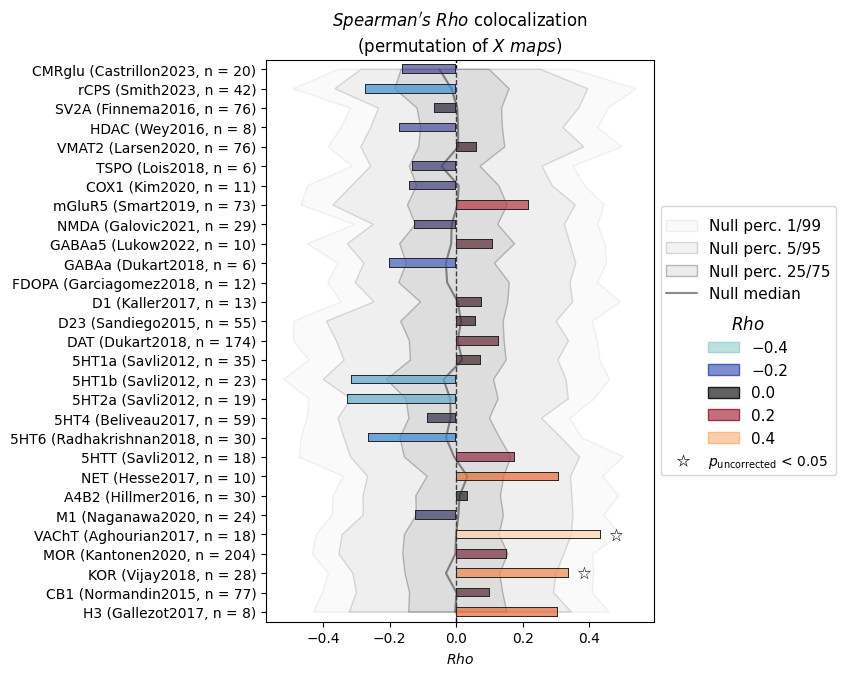
nsp.plot() can incorporate any of the correction methods. Pass mc_method to display corrected significance annotations:

[8]:

nsp.plot(mc_method="meff")

INFO | 01/06/26 15:04:05 | nispace.plotting: Significance annotation: 2/29 p_uncorrected < 0.05, 0/29 p_meff < 0.05

../_images/nb_introduction_intro06_multiple_comparisons_15_1.png

[8]:

(<Figure size 500x730 with 1 Axes>,
 <Axes: title={'center': "$Spearman's\\ Rho$ colocalization\n(permutation of $X\\ maps$)"}, xlabel='$Rho$'>,
 <seaborn._core.plot.Plotter at 0x15e727f40>)

Which method should I use?

Meff (default): The NiSpace default and the right starting point for most analyses. It accounts for the actual correlation structure of your reference maps and is more powerful than Bonferroni without any additional assumptions.
maxT / step-maxT: Excellent alternatives when your colocalization method produces statistics on a comparable scale — that is, Spearman or Pearson correlations, or regression with z-scored X. Computationally free once permute() has run. Step-maxT has more power than basic maxT.
FDR-BH: Appropriate when you’re comfortable with FDR control rather than FWER — common in exploratory neuroimaging but note that the interpretation differs.
Bonferroni: Rarely justified; Meff is strictly better when your tests are correlated, which they typically are for any standard reference dataset.

Summary

Method	Call	Controls
Meff — NiSpace default	`nsp.correct_p()`	FWER
maxT	`nsp.correct_p(mc_method="maxT")`	FWER
step-maxT	`nsp.correct_p(mc_method="step_maxT")`	FWER
FDR (Benjamini-Hochberg)	`nsp.correct_p(mc_method="fdr_bh")`	FDR
Bonferroni	`nsp.correct_p(mc_method="bonferroni")`	FWER

Retrieve corrected p-values with nsp.get_p_values(mc_method=...) after calling correct_p().

Next: Notebook 7 covers how to customize NiSpace.plot() and NiSpace.plot_brain() to produce publication-quality figures.